3.1: Exponential and Logistic Applications

There are a variety of different types of mathematical relationships. The simplest mathematical relationship is the additive relationship. This is a situation in which the value of one quantity is always a certain amount more (or less) than another quantity. A good example of an additive relationship is an age relationship. In an age relationship, the age of the older person is always the same amount more than the age of the younger person. If the older person is five years older, then the age of the older person ( ) will always be equal to the age of the younger person plus five:

Another type of additive relationship is seen where two quantities add up to a constant value. Let's say there is a board whose length is 20 inches. If we cut it into two pieces, with one piece being 6 inches, then the other piece will be 14 inches. If one piece is 9 inches, then the other will be 11 inches. If one piece is inches, then the other piece will be or

The next type of mathematical relationshp is a multiplicative relationship. This represents a situation in which one quantity is always a multiple of the other quantity. This is commonly seen in proportional relationships. If a recipe for a cake calls for 2 cups of flour, then, if we want to make 3 cakes, we'll need 6 cups of flour. The amount of flour is always two times the number of cakes we want to make

If a recipe for a batch of cookies (with 20 cookies per batch) calls for 1.5 cups of sugar, then three batches would require 4.5 cups of sugar. The amount of sugar required ( ) is always the number of batches times . If we wanted to represent this relationship based on the number of cookies instead of the number of batches, we would need to adjust the formula. Given that there are 20 cookies per batch, we could adjust our formula so that we first calculate the number of batches from the number of cookies and then multiply by If the number of cookies is and the amount of sugar is then or
The next type of mathematical relationship is the polynomial relationship. In this type of relationship, one quantity is related to a power of another quantity. A good example of this type of relationship involves gravity. As Galileo discovered in the 16 th century, the distance that an object falls after it is dropped is not proportional to the time that it has been falling. Rather, it is proportional to the square of the time. The table below shows this type of relationship.

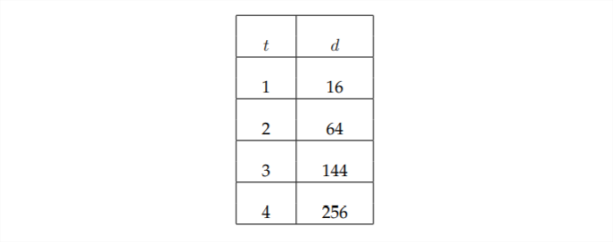
After one second, it looks like the distance will always be sixteen times the time the object has been falling. However, after two seconds, we can see that this relationship no longer is true. That's because this relationship is a polynomial relationship in which the distance an object has fallen ( ) is proportional to the square of the time it has been falling

Exponential Relationships
The next type of relationship is the focus of this chapter - the exponential relationship. In this situation, the rate of change of a quantity is proportional to the size of that quantity. This relationship can be explored in more depth in an integral calculus course, but we will discuss the basics here.

In a linear or proportional relationship, the slope, or rate of change, is constant. For example, in the equation the slope is always three, no matter what the values of and are. In an exponential relationship, the rate of change (also called " prime" or ) is proportional to the value of In this case, we say that

This is what is known as a differential equation. This is an equation in which the variable and its rate of change are related. Through the processes of differential and integral calculus, we can solve the equation above as:

In the equation above, is the value of at time is a constant that determines how fast the quantity increases or decreases and plays the role of the independent variable (as often does) and represents the time that has passed. If is positive, then the quantity is growing because its rate of change is positive. If is negative, then the quantity is decreasing because the rate of change is negative.

The quantity represented by in the above equation is a mathematical constant (like ) that is often used to represent exponential relationships. The best way to understand the value of and what it represents is directly related to fundamental questions from differential and integral calculus.

Differential Calculus is concerned primarily with the question of slopes. We discussed earlier that a linear relationship has a constant slope. Polynomial and exponential relationships have slopes that depend on the value of and / or . This is what makes them curves rather than lines. If we consider the slopes of some different exponential relationships, we can see one aspect of where the value for comes from.

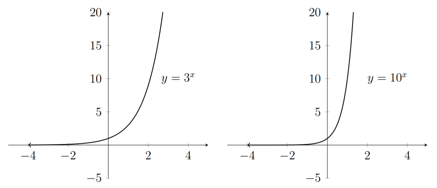
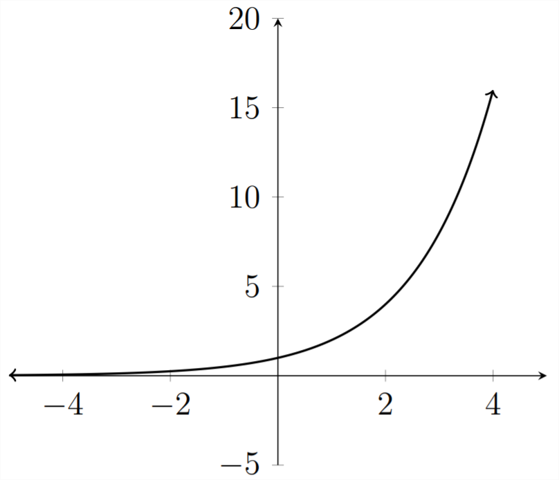
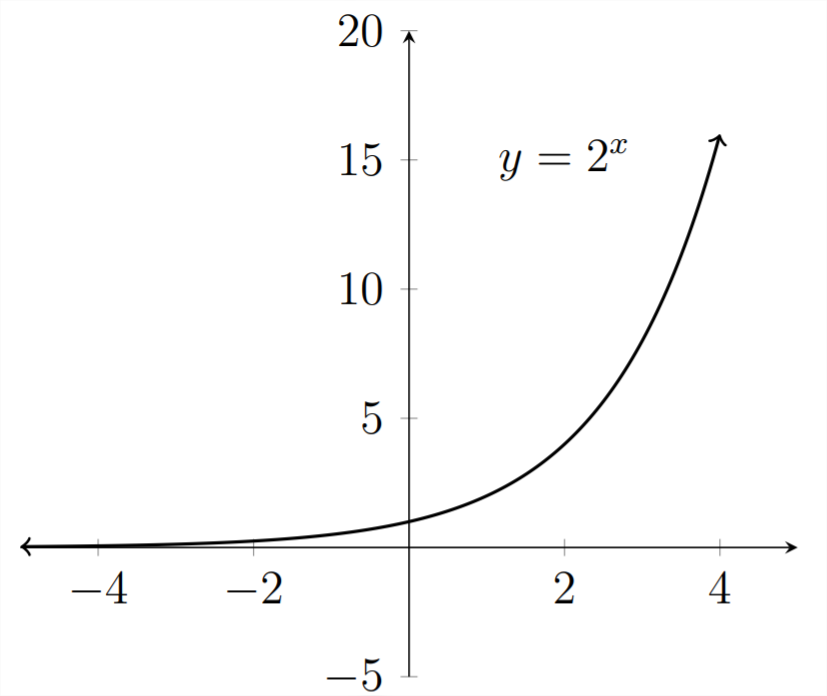
Consider the graphs of the following relationships:

Let's look at the graphs for these functions:


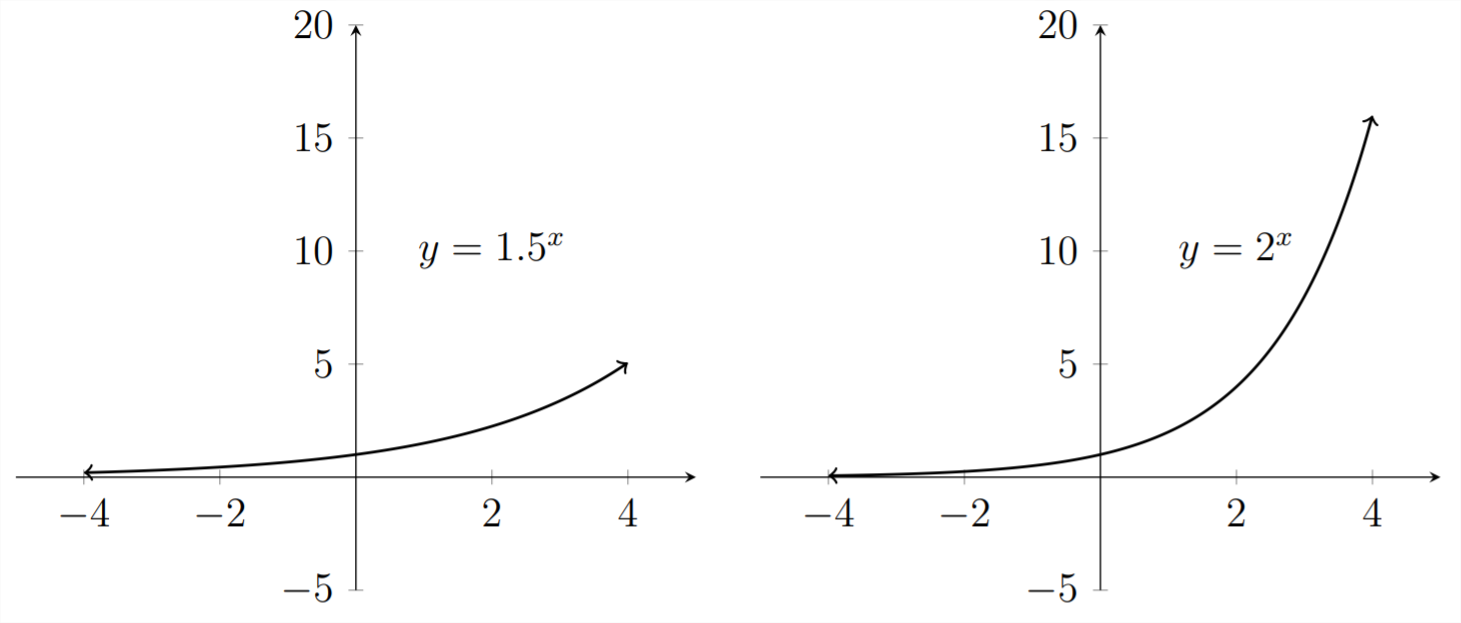
We can see that these graphs demonstrate slightly different behavior and different and values. One thing that they all have in common is that they all pass through the point (0,1) on the graph. This is because and Therefore the point where is 0 and is 1 is on all four of the graphs.
Although all four of the graphs pass through the point they each do this in a different way. Let's look at the slope of a line tangent to each curve at the point This is the straight line that touches the curve at the point but nowhere else:


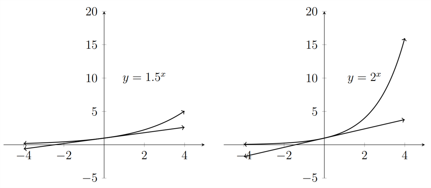
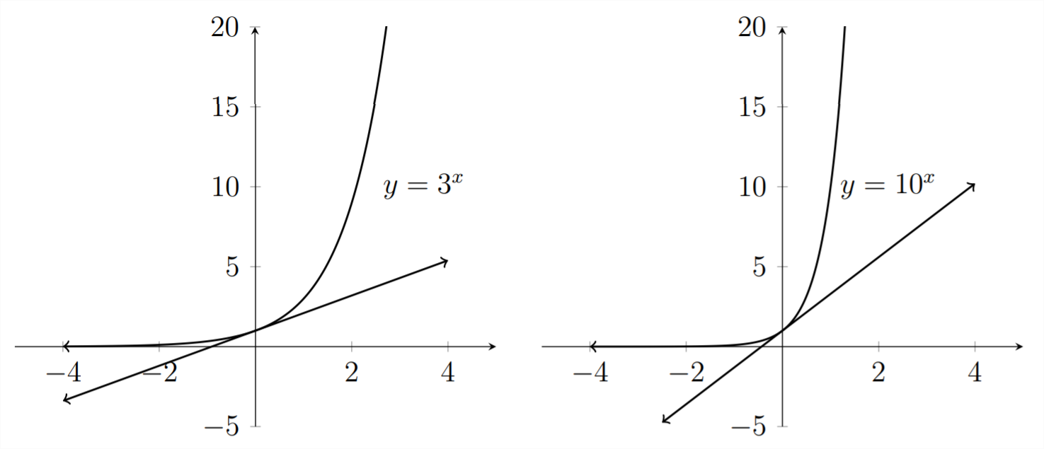
We can see that the slopes of these tangent lines are all different. In the case of the slope of the tangent line at (0,1) is about while for the graph of the slope of the tangent line at (0,1) is about 1.1

As mathematicians examined these graphs during the 17 th and 18 th centuries, they began to question what the value of the base " should be in the equation so that the slope of the tangent line at the point (0,1) would be equal to exactly The answer was

Another way to derive the value of uses Integral Calculus. Integral Calculus is often concerned with finding the area under a curve. This process can then be generalized and used to make many other types of calculations that are similar to finding area.
Consider the graph of the curve

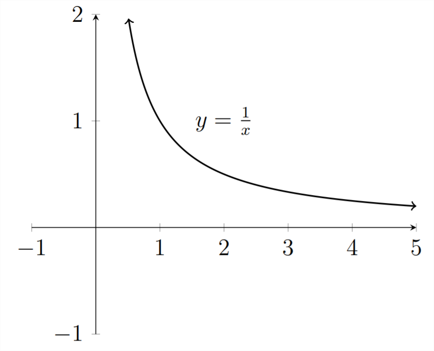
We can delineate borders on the values and determine the area of the resulting region using the techniques of calculus:

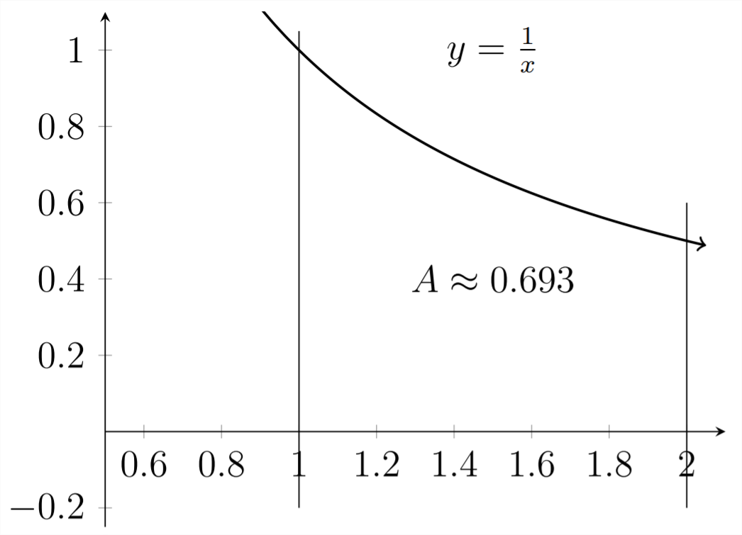
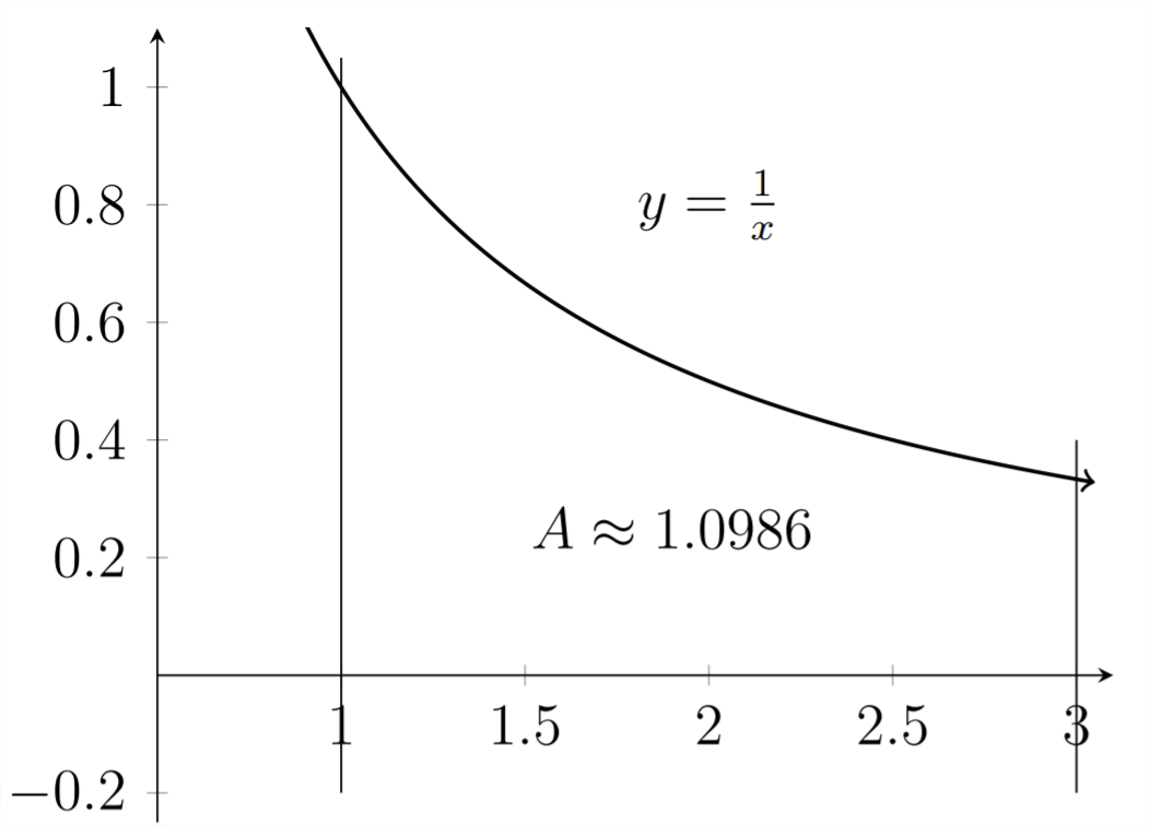
These values for the area under the curve are actually the same values as those for the slope of the tangent line in the previous graphs. If you ask the question, "Where should you draw the second vertical line so that the area under the curve is equal to exactly then just like the slope question, the answer is
This is how the value of was determined and why it is used to represent these exponential relationships.

Logistic Relationships
Let's consider the graph of

If we extend the -axis out further past we would see that the values for this relationship will grow very quickly, as they continue doubling.

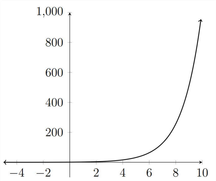
Some phenomena in the natural world exhibit behavior similar to the growth of this function. However, in the natural world, few, if any, things can grow unconstrained. Most growth of any kind is limited by the resources that fuel the growth. Populations often grow exponentially for a period of time, however, populations are dependent on natural resources to continue growing. As a result, the simple exponential function is only useful for modeling real-world behavior if the -values are limited.

It was this problem with the simple exponential function that led French mathematician Pierre Verhulst to slightly adjust the differential equation that gives rise to the exponential function to make it more realistic.
The original differential equation said:

This says that the rate of growth of is always directly proportional to the value of
In other words the larger a population gets, the faster it will grow - forever. Verhulst changed this to say:

This is the defining relationship for the Logistic function. Notice that when values of are small, this is essentially the same as the simple exponential. If is small, then the term will be very close to 1 and will produce behavior very much like the simple exponential.

The in the formula is a theoretical "maximum population." As the value of approaches this maximum value, will approach 1 and will get smaller and smaller. As it gets smaller, the factor of will slow down the growth of the function to model the pressure that is put on the resources that are driving the growth.

The solution of the Logistic equation is quite complicated and results in a standard form of:

The graph for a sample logistic relationship is shown below:

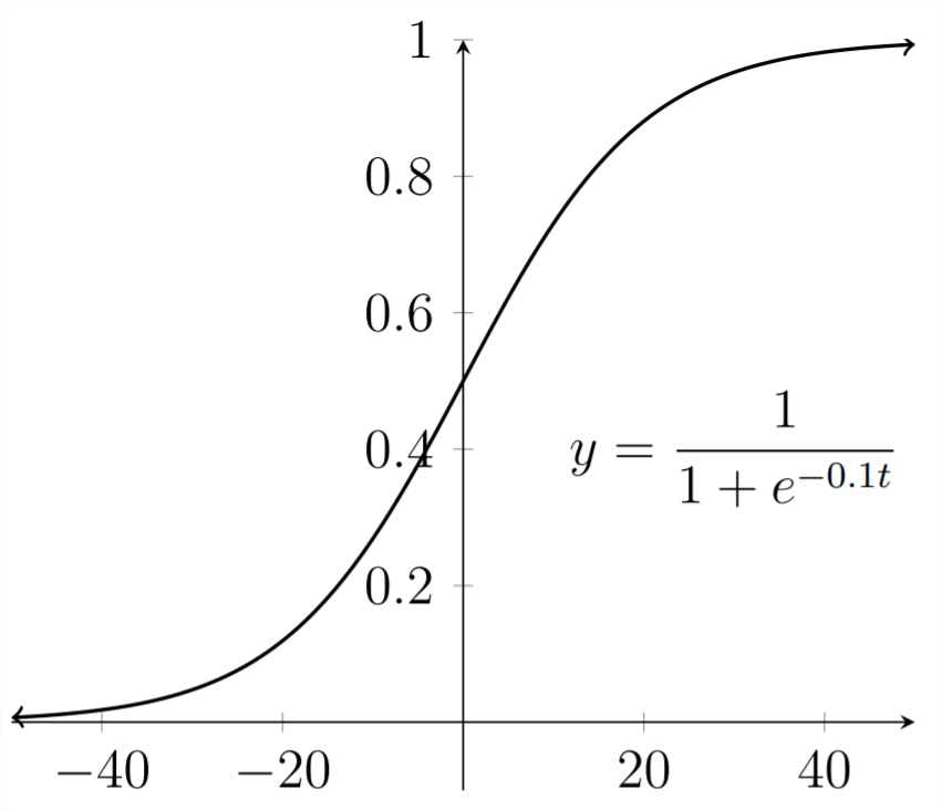
The "lazy-s" shape is characteristic of the logistic function. In the early stages, the relationship shows growth very similar to the simple exponential function but, as the function grows larger, the growth decreases and the function values stabilize. The maximum value of is always the horizontal asymptote for the logistic function.

Negative Exponential Relationships
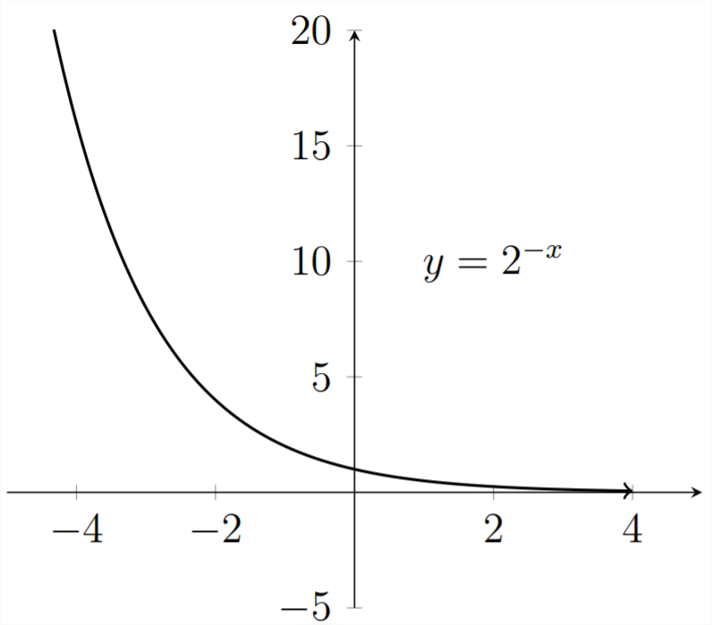
The Logistic function is very useful for modeling phenomena from the natural world. Although the simple exponential function is somewhat limited in modeling natural phenomena, the negative exponential is quite useful. Looking back to the graph of :

If we turn the graph around by changing to in the formula, then we will be working with the decaying tail of the graph:

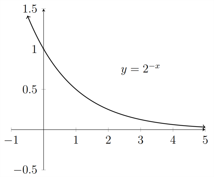
Let's zoom in on the portion of the graph in the Quadrant I:

The behavior shown in the graph is quite useful for modeling radioactive decay, processes of heating and cooling, and assimilation of medication in the bloodstream. Let's look at an example.

Example
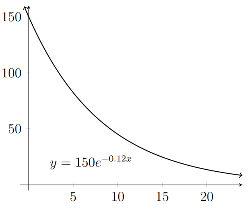
If a patient is injected with 150 micrograms of medication, the amount of medication still in the bloodstream after hours is given by the function:

a) Find the amount of medication in the bloodstream after 3 hours.
Round your answer to the nearest 100 th.
b) How long will it take for the amount of medication to reach 60 micrograms?
Round your answer to the nearest 10 th of an hour.

In this section we will focus on solving these problems using the graphing calculator. In later sections, we will cover processes that can be used to solve these problems algebraically. It is helpful to understand both methods of solution.
First, let's graph the function given in the problem:

We can directly calculate the answer for part
(a) by plugging the value of 3 for or we can use the table in the graphing calculator to find this value:

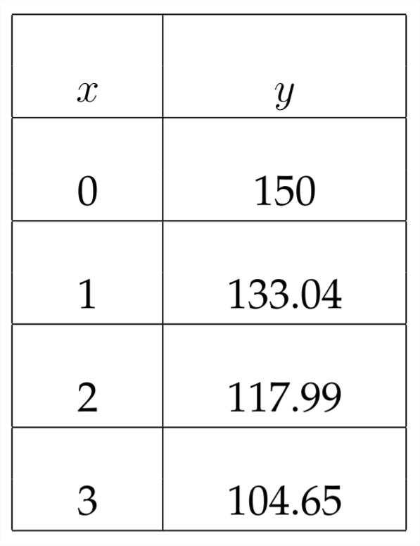
We can see that after 3 hours there are approximately 104.65 micrograms of medication in the patient's bloodstream.

To answer part (b) graphically, we'll graph the original function along with the horizontal line When we find the intersection of these two graphs, we'll know how long it takes for there to be 60 micrograms of medication in the patient's bloodstream:

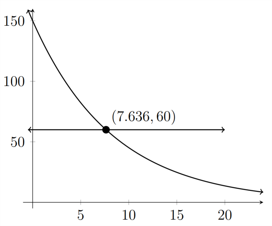
Here, we can see that it would take about 7.6 hours (or about 7 hours 36 minutes), for there to be 60 micrograms of medication in the patient's bloodstream.

Example
The deer population on a nature preserve can be modeled using the equation:

indicates the number of deer living in the nature preserve and represents the number of years that have passed since the initial population of deer were established there.
a) How many deer were in the initial population?
b) What is the deer population after 10 years?
Round your answer to the nearest whole number.
c) How long does it take for the population to reach
Round your answer to the nearest 10 th of a year.
Parts
(a) and (b) can both be answered from a table of values for the function. Before we look at the table, let's consider the question in Part (a). The problem is asking what the initial population of deer was. The means that we're looking to find out what is when
Let's see what happens when we plug zero in for in the formula:

Let's look at the table of values:

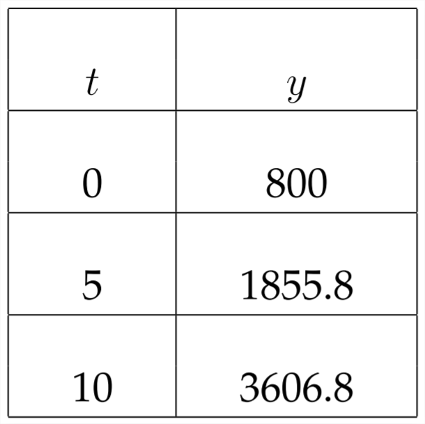
To the nearest whole number, the deer population after 10 years is 3,607
In Part (c), we'll need to graph a horizontal line at and find the intersection.


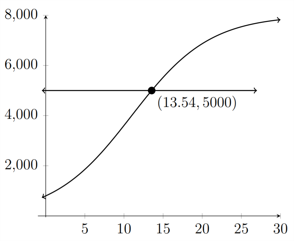
To the nearest 10 th, it takes about 13.5 years for the deer population to reach 5,000

Exercises 3.1
1) Medication in the bloodstream
The function gives the amount of medication, in milligrams, in a patient's bloodstream minutes after the medication has been injected.
a) Find the amount of medication in the bloodstream after 45 minutes.
Round your answer to the nearest milligram.
b) How long will it take for the amount of medication to reach 50 milligrams?
Round your answer to the nearest minute.

2) Medication in the bloodstream
The function gives the amount of medication, in milligrams, in a patient's bloodstream hours after the medication has been injected.
a) Find the amount of medication in the bloodstream after 3 hours.
Round your answer to the nearest milligram.
b) How long will it take for the amount of medication to reach 10 milligrams?
Round your answer to the nearest minute.

3) Fish Population
The number of bass in a lake can be modeled using the given equation:

where is the number of months that have passed since the lake was stocked with bass. In each question below, round your answer to the nearest whole number.
a) How many bass were in the lake immediately after it was stocked?
b) How many bass were in the lake 1 year after it was stocked?

4) Bird Population
The population of a certain species of bird is limited by the type of habitat required for nesting. The population can be modeled using the following equation:

where is the number of years. In each question below, round your answer to the nearest whole number.
a) Find the initial bird population.
b) What is the population 100 years later?

5) A Temperature Model
A cup of coffee is heated to and placed in a room that maintains a temperature of . The temperature of the coffee after minutes have passed is given by:

a) Find the temperature of the coffee 10 minutes after it is placed in the room.
Round your answer to the nearest degree.
b) When will the temperature of the coffee be ?
Round your answer to the nearest tenth of a minute.

6) A Temperature Model
Soup at a temperature of is poured into a bowl in a room that maintains a constant temperature. The temperature of the soup decreases according to the model given by:

where is the number of minutes that have passed since the soup was poured.
a) What is the temperature of the soup after 2 minutes?
Round your answer to the nearest 10 th of a degree.
b) A certain customer prefers that the soup be cooled to .
How long will this take?
Round your answer to the nearest 10 th of a minute.

7) Radioactive Decay
A radioactive substance decays in such a way that the amount of mass remaining after days is given by the equation:

where the amount is measured in kilograms.
a) Find the mass at time
b) How much of the mass remains after 45 days?
c) How long does it take for there to be 5 kg. left?

8) Radioactive Decay
Radioactive iodine is used by doctors as a tracer in diagnosing certain thyroid gland disorders. This type of iodine decays in such a way that the mass remaining after days is given by:

where the amount is measured in grams.
a) Find the mass at time
b) How much remains after 20 days?
c) How long does it take for there to be 2 grams left?
Round your answer to the nearest tenth of a day.

9) Fish population
The function:

gives the size of a fish population in thousands at time measured in years.
a) Find the initial population of fish at time
Find the population of fish after 2 years, time
b) How long will it take for the population to be
What appears to be the maximum population for this particular model?

10) Fish population
The function:

gives the size of a fish population in thousands at time measured in years.
a) Find the initial population of fish at time
Find the population of fish after 1.5 years,
b) How long will it take for the population to be
What appears to be the maximum population for this particular model?

11) Fish population
The function:

gives the size of a fish population in thousands at time measured in years.
a) Find the initial population of fish at time
Find the population of fish after 5 years, time
b) How long will it take for the population to be
What happens to this population over time?

12) Fish population
The function:

gives the size of a fish population in thousands at time measured in years.
a) Find the initial population of fish at time
Find the population of fish after 5 years, time
b) How long will it take for the population to be
What happens to this population over time?

13) Continuous Mixing
A 100 gallon tank of pure water has salt water with 0.5 lb per gallon added to it at a rate of 2 gallons per minute. The brine solution is mixed thoroughly and drained at rate of 2 gallons per minute.

The equation for how many pounds of salt are in the tank at time is given by:

where is measured in pounds and is measured in minutes.
a) How many pounds of salt are in the tank after 20 minutes?
b) How long does it take for there to be 30 lbs of salt in the tank?
Round your answer to the nearest tenth of a minute.

14) Continuous Mixing
A 20 gallon tank of pure water has salt water with 0.4 lb per gallon of salt added to it at a rate of 3 gallons per minute. The brine solution is mixed thoroughly and drained at rate of 3 gallons per minute.

The equation for how many pounds of salt are in the tank at time is given by:

where is measured in pounds and is measured in minutes.
a) How many pounds of salt are in the tank after 15 minutes?
b) How long does it take for there to be 6 lbs of salt in the tank?
Round your answer to the nearest tenth of a minute.

15) Continuous Mixing
A tank contains 200 gallons of a solution of HCl. A solution of HCl is added at 5 gallons per minute. The well mixed solution is being drained at 5 gallons per minute.
The amount of HCl in the tank at any given time in minutes is:

a) How many gallons of HCl are in the tank at minutes?
b) When does the concentration of HCl in the solution reach

16) Continuous Mixing
A tank contains 100 gallons of salt water which contains a total of 25 lbs of salt. Salt water containing 0.4 lbs per gallon is added to the tank at a rate of 5 gallons per minute and the well-mixed solution is drained at the same rate.
The amount of salt in pounds in the tank at any given time in minutes is:

a) How many pounds of salt are in the tank at minutes?
b) How long does it take for there to be 30 lbs of salt in the tank?