4.2: Domain and Range of a Function

Last updated
Save as PDF

Page ID: 40915

$ \newcommand{\vecs}[1]{\overset { \scriptstyle \rightharpoonup} {\mathbf{#1}} } $ $ \newcommand{\vecd}[1]{\overset{-\!-\!\rightharpoonup}{\vphantom{a}\smash {#1}}} $$\newcommand{\id}{\mathrm{id}}$ $ \newcommand{\Span}{\mathrm{span}}$ $ \newcommand{\kernel}{\mathrm{null}\,}$ $ \newcommand{\range}{\mathrm{range}\,}$ $ \newcommand{\RealPart}{\mathrm{Re}}$ $ \newcommand{\ImaginaryPart}{\mathrm{Im}}$ $ \newcommand{\Argument}{\mathrm{Arg}}$ $ \newcommand{\norm}[1]{\| #1 \|}$ $ \newcommand{\inner}[2]{\langle #1, #2 \rangle}$ $ \newcommand{\Span}{\mathrm{span}}$ $\newcommand{\id}{\mathrm{id}}$ $ \newcommand{\Span}{\mathrm{span}}$ $ \newcommand{\kernel}{\mathrm{null}\,}$ $ \newcommand{\range}{\mathrm{range}\,}$ $ \newcommand{\RealPart}{\mathrm{Re}}$ $ \newcommand{\ImaginaryPart}{\mathrm{Im}}$ $ \newcommand{\Argument}{\mathrm{Arg}}$ $ \newcommand{\norm}[1]{\| #1 \|}$ $ \newcommand{\inner}[2]{\langle #1, #2 \rangle}$ $ \newcommand{\Span}{\mathrm{span}}$$\newcommand{\AA}{\unicode[.8,0]{x212B}}$

The analysis of the behavior of functions addresses questions of when the function is increasing or decreasing, whether and where it has maximum or minimum values, where it crosses the $x$ or $y$ axis, and which values of $x$ and $y$ are to be included in the function.

The set of values available for the $x,$ or independent variable is called the Domain of the function. The set of corresponding $y$ values is called the Range of the function.

The linear function mentioned above $f(x)=6 x-1$ has a domain of all real numbers and a range of all real numbers, $x \in \mathbb{R}$ and $y \in \mathbb{R}$. On the other hand, the function $f(x)=x^{2}$ has a domain of all real numbers, $x \in \mathbb{R},$ but its range is limited to the positive real numbers, $y \geq 0$

Considerations of the domain of a function typically refer to restrictions on which $x$ values will generate real number values for $y .$ The most common restrictions occur with the use of square root functions or rational functions.

The domain of the function $f(x)=\sqrt{x-7}$ would be the set of $x \geq 7,$ so that no negative values are permitted under the square root. This secures the necessary real values for $y .$ The range for this function is $y \geq 0$

The domain of the function $f(x)=\frac{x}{2 x-3}$ would be $x \in \mathbb{R}$ (all real numbers), but $x \neq \frac{3}{2},$ thus avoiding a zero denominator which is an undefined value. The range for this function would be $y \in \mathbb{R}$ (all real numbers), but $y \neq \frac{1}{2},$ due to the horizontal asymptote at $y=\frac{1}{2}$

The questions of domain and range become more interesting when considered in relation to functions defined by graphs, or in applications. In an application involving perimeter in which the perimeter of a rectangle is given as 50 feet, we know that
\[
2 \ell+2 w=50
\]
Rewriting this as a function of $w,$ we can say that
\[
\ell=f(w)=25-w
\]

In this function relating the length and width based on a given perimeter, we can say the domain of the function is $0<w<25 .$ The width must be greater than 0 but less than $25,$ otherwise there would not be a rectangle. The same is true for the range or possible set of values for the length $0<\ell<25$Exercises 4.2
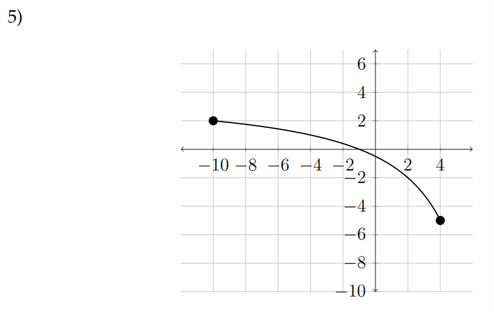
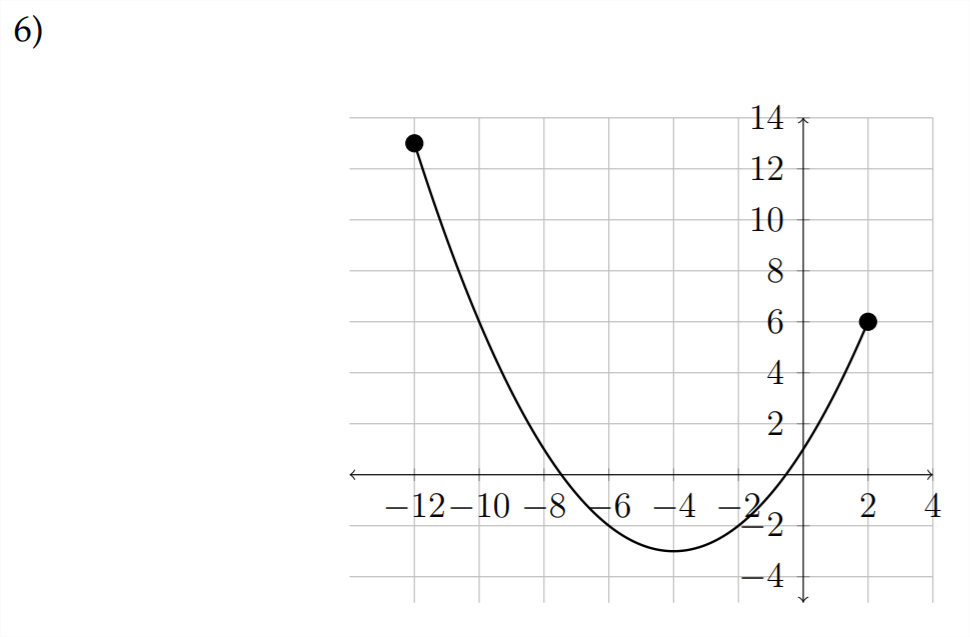
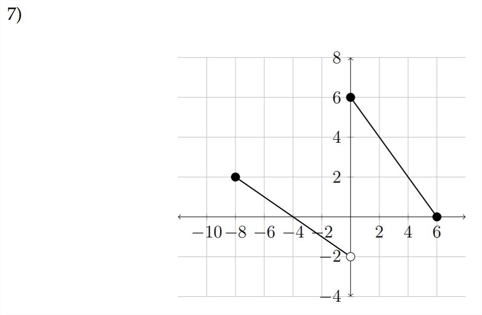
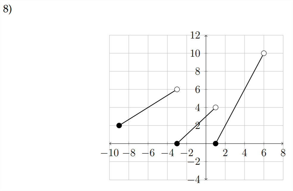
Find the domain and range for each of the following functions:
1) $\quad f(x)=\sqrt{2 x+1}$
2) $\quad f(x)=\sqrt{3 x-5}$
3) $\quad \frac{x}{x+9}$
4) $\quad f(x)=\frac{x+2}{2 x-3}$
For the following graphs, assume that the endpoints for the domain and range are whole numbers.
$clipboard_ede5b848f28fbb4845ea8769b35bfeb79.png$
$clipboard_e63f6320a00d3ae34202efb85c8dce51f.png$
$clipboard_e3f0e1f16d5e111f7a4e5312c52626118.png$
$clipboard_e27936a7a141f7f0d7bd275397eedc54b.png$