
2.2: The Graph of a Function
- Page ID
- 19686

\( \newcommand{\vecs}[1]{\overset { \scriptstyle \rightharpoonup} {\mathbf{#1}} } \)
\( \newcommand{\vecd}[1]{\overset{-\!-\!\rightharpoonup}{\vphantom{a}\smash {#1}}} \)
\( \newcommand{\dsum}{\displaystyle\sum\limits} \)
\( \newcommand{\dint}{\displaystyle\int\limits} \)
\( \newcommand{\dlim}{\displaystyle\lim\limits} \)
\( \newcommand{\id}{\mathrm{id}}\) \( \newcommand{\Span}{\mathrm{span}}\)
( \newcommand{\kernel}{\mathrm{null}\,}\) \( \newcommand{\range}{\mathrm{range}\,}\)
\( \newcommand{\RealPart}{\mathrm{Re}}\) \( \newcommand{\ImaginaryPart}{\mathrm{Im}}\)
\( \newcommand{\Argument}{\mathrm{Arg}}\) \( \newcommand{\norm}[1]{\| #1 \|}\)
\( \newcommand{\inner}[2]{\langle #1, #2 \rangle}\)
\( \newcommand{\Span}{\mathrm{span}}\)
\( \newcommand{\id}{\mathrm{id}}\)
\( \newcommand{\Span}{\mathrm{span}}\)
\( \newcommand{\kernel}{\mathrm{null}\,}\)
\( \newcommand{\range}{\mathrm{range}\,}\)
\( \newcommand{\RealPart}{\mathrm{Re}}\)
\( \newcommand{\ImaginaryPart}{\mathrm{Im}}\)
\( \newcommand{\Argument}{\mathrm{Arg}}\)
\( \newcommand{\norm}[1]{\| #1 \|}\)
\( \newcommand{\inner}[2]{\langle #1, #2 \rangle}\)
\( \newcommand{\Span}{\mathrm{span}}\) \( \newcommand{\AA}{\unicode[.8,0]{x212B}}\)
\( \newcommand{\vectorA}[1]{\vec{#1}} % arrow\)
\( \newcommand{\vectorAt}[1]{\vec{\text{#1}}} % arrow\)
\( \newcommand{\vectorB}[1]{\overset { \scriptstyle \rightharpoonup} {\mathbf{#1}} } \)
\( \newcommand{\vectorC}[1]{\textbf{#1}} \)
\( \newcommand{\vectorD}[1]{\overrightarrow{#1}} \)
\( \newcommand{\vectorDt}[1]{\overrightarrow{\text{#1}}} \)
\( \newcommand{\vectE}[1]{\overset{-\!-\!\rightharpoonup}{\vphantom{a}\smash{\mathbf {#1}}}} \)
\( \newcommand{\vecs}[1]{\overset { \scriptstyle \rightharpoonup} {\mathbf{#1}} } \)
\(\newcommand{\longvect}{\overrightarrow}\)
\( \newcommand{\vecd}[1]{\overset{-\!-\!\rightharpoonup}{\vphantom{a}\smash {#1}}} \)
\(\newcommand{\avec}{\mathbf a}\) \(\newcommand{\bvec}{\mathbf b}\) \(\newcommand{\cvec}{\mathbf c}\) \(\newcommand{\dvec}{\mathbf d}\) \(\newcommand{\dtil}{\widetilde{\mathbf d}}\) \(\newcommand{\evec}{\mathbf e}\) \(\newcommand{\fvec}{\mathbf f}\) \(\newcommand{\nvec}{\mathbf n}\) \(\newcommand{\pvec}{\mathbf p}\) \(\newcommand{\qvec}{\mathbf q}\) \(\newcommand{\svec}{\mathbf s}\) \(\newcommand{\tvec}{\mathbf t}\) \(\newcommand{\uvec}{\mathbf u}\) \(\newcommand{\vvec}{\mathbf v}\) \(\newcommand{\wvec}{\mathbf w}\) \(\newcommand{\xvec}{\mathbf x}\) \(\newcommand{\yvec}{\mathbf y}\) \(\newcommand{\zvec}{\mathbf z}\) \(\newcommand{\rvec}{\mathbf r}\) \(\newcommand{\mvec}{\mathbf m}\) \(\newcommand{\zerovec}{\mathbf 0}\) \(\newcommand{\onevec}{\mathbf 1}\) \(\newcommand{\real}{\mathbb R}\) \(\newcommand{\twovec}[2]{\left[\begin{array}{r}#1 \\ #2 \end{array}\right]}\) \(\newcommand{\ctwovec}[2]{\left[\begin{array}{c}#1 \\ #2 \end{array}\right]}\) \(\newcommand{\threevec}[3]{\left[\begin{array}{r}#1 \\ #2 \\ #3 \end{array}\right]}\) \(\newcommand{\cthreevec}[3]{\left[\begin{array}{c}#1 \\ #2 \\ #3 \end{array}\right]}\) \(\newcommand{\fourvec}[4]{\left[\begin{array}{r}#1 \\ #2 \\ #3 \\ #4 \end{array}\right]}\) \(\newcommand{\cfourvec}[4]{\left[\begin{array}{c}#1 \\ #2 \\ #3 \\ #4 \end{array}\right]}\) \(\newcommand{\fivevec}[5]{\left[\begin{array}{r}#1 \\ #2 \\ #3 \\ #4 \\ #5 \\ \end{array}\right]}\) \(\newcommand{\cfivevec}[5]{\left[\begin{array}{c}#1 \\ #2 \\ #3 \\ #4 \\ #5 \\ \end{array}\right]}\) \(\newcommand{\mattwo}[4]{\left[\begin{array}{rr}#1 \amp #2 \\ #3 \amp #4 \\ \end{array}\right]}\) \(\newcommand{\laspan}[1]{\text{Span}\{#1\}}\) \(\newcommand{\bcal}{\cal B}\) \(\newcommand{\ccal}{\cal C}\) \(\newcommand{\scal}{\cal S}\) \(\newcommand{\wcal}{\cal W}\) \(\newcommand{\ecal}{\cal E}\) \(\newcommand{\coords}[2]{\left\{#1\right\}_{#2}}\) \(\newcommand{\gray}[1]{\color{gray}{#1}}\) \(\newcommand{\lgray}[1]{\color{lightgray}{#1}}\) \(\newcommand{\rank}{\operatorname{rank}}\) \(\newcommand{\row}{\text{Row}}\) \(\newcommand{\col}{\text{Col}}\) \(\renewcommand{\row}{\text{Row}}\) \(\newcommand{\nul}{\text{Nul}}\) \(\newcommand{\var}{\text{Var}}\) \(\newcommand{\corr}{\text{corr}}\) \(\newcommand{\len}[1]{\left|#1\right|}\) \(\newcommand{\bbar}{\overline{\bvec}}\) \(\newcommand{\bhat}{\widehat{\bvec}}\) \(\newcommand{\bperp}{\bvec^\perp}\) \(\newcommand{\xhat}{\widehat{\xvec}}\) \(\newcommand{\vhat}{\widehat{\vvec}}\) \(\newcommand{\uhat}{\widehat{\uvec}}\) \(\newcommand{\what}{\widehat{\wvec}}\) \(\newcommand{\Sighat}{\widehat{\Sigma}}\) \(\newcommand{\lt}{<}\) \(\newcommand{\gt}{>}\) \(\newcommand{\amp}{&}\) \(\definecolor{fillinmathshade}{gray}{0.9}\)Rene Descartes (1596-1650) was a French philosopher and mathematician who is well known for the famous phrase “cogito ergo sum” (I think, therefore I am), which appears in his Discours de la methode pour bien conduire sa raison, et chercher la verite dans les sciences (Discourse on the Method of Rightly Conducting the Reason, and Seeking Truth in the Sciences). In that same treatise, Descartes introduces his coordinate system, a method for representing points in the plane via pairs of real numbers. Indeed, the Cartesian plane of modern day is so named in honor of Rene Descartes, who some call the “Father of Modern Mathematics.”
Descartes’ work, which forever linked geometry and algebra, was continued in an appendix to Discourse on Method, entitled La Geometrie, which some consider the beginning of modern mathematics. Certainly both Newton and Leibniz, in developing the Calculus, built upon the foundation provided in this work by Descartes.
A Cartesian Coordinate System consists of a pair of axes, usually drawn at right angles to one another in the plane, one horizontal (labeled x) and one vertical (labeled y), as shown in the Figure \(\PageIndex{1}\). The quadrants are numbered I, II, III, and IV, in counterclockwise order, and samples of ordered pairs of the form (x, y) are shown in each quadrant of the Cartesian coordinate system in Figure \(\PageIndex{1}\).
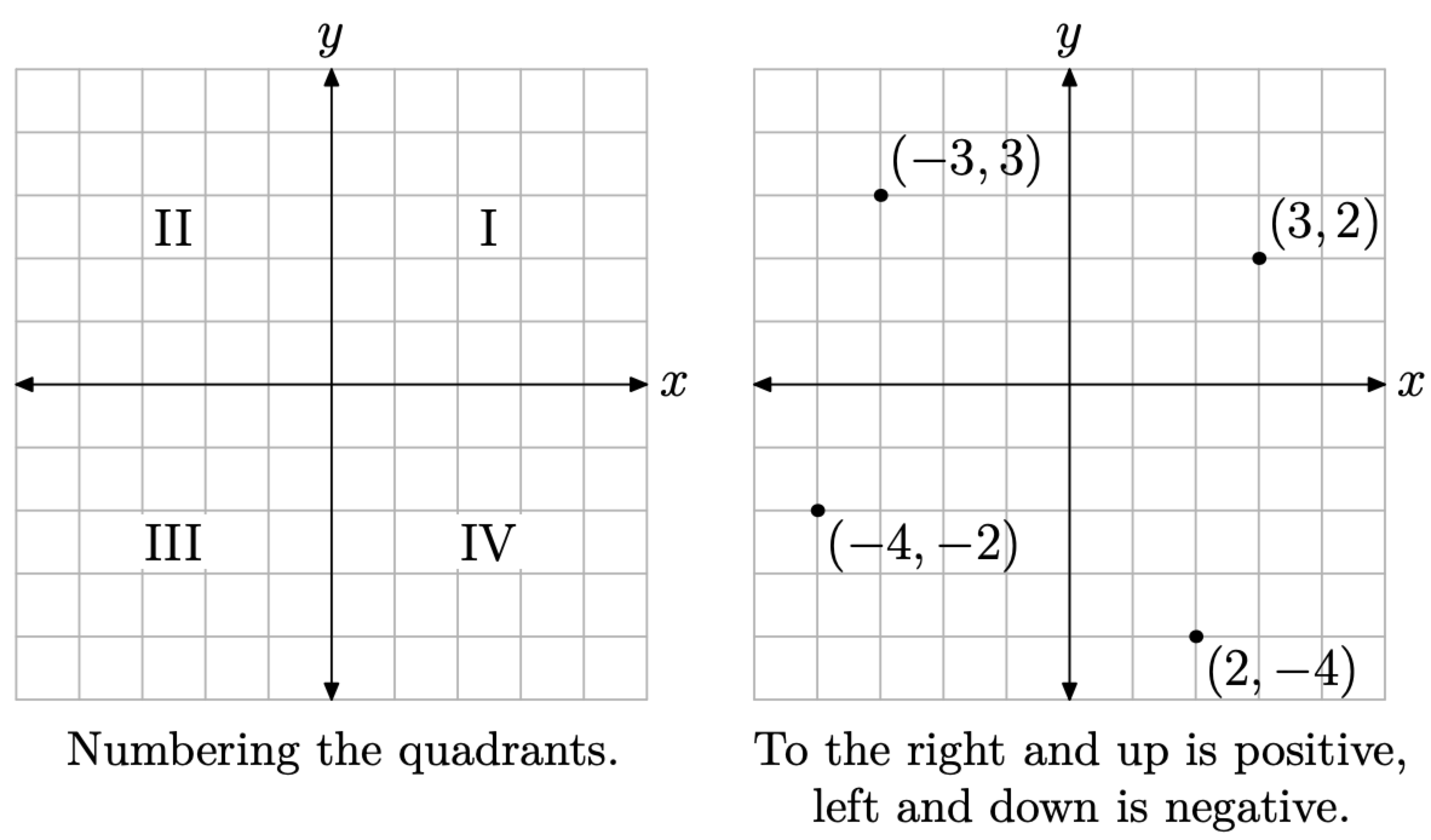
Figure \(\PageIndex{1}\). The Cartesian coordinate system.
Now, suppose that we have a relation \[R=\{(1,2),(3,1),(3,4),(4,3)\} \nonumber \]
Recall that relation is the name given to a collection of ordered pairs. In Figure \(\PageIndex{2}\)(b) we’ve plotted each of the ordered pairs in the relation R. This is called the graph of the relation R.
The graph of a relation is the collection of all ordered pairs of the relation. These are usually represented as points in a Cartesian coordinate system.
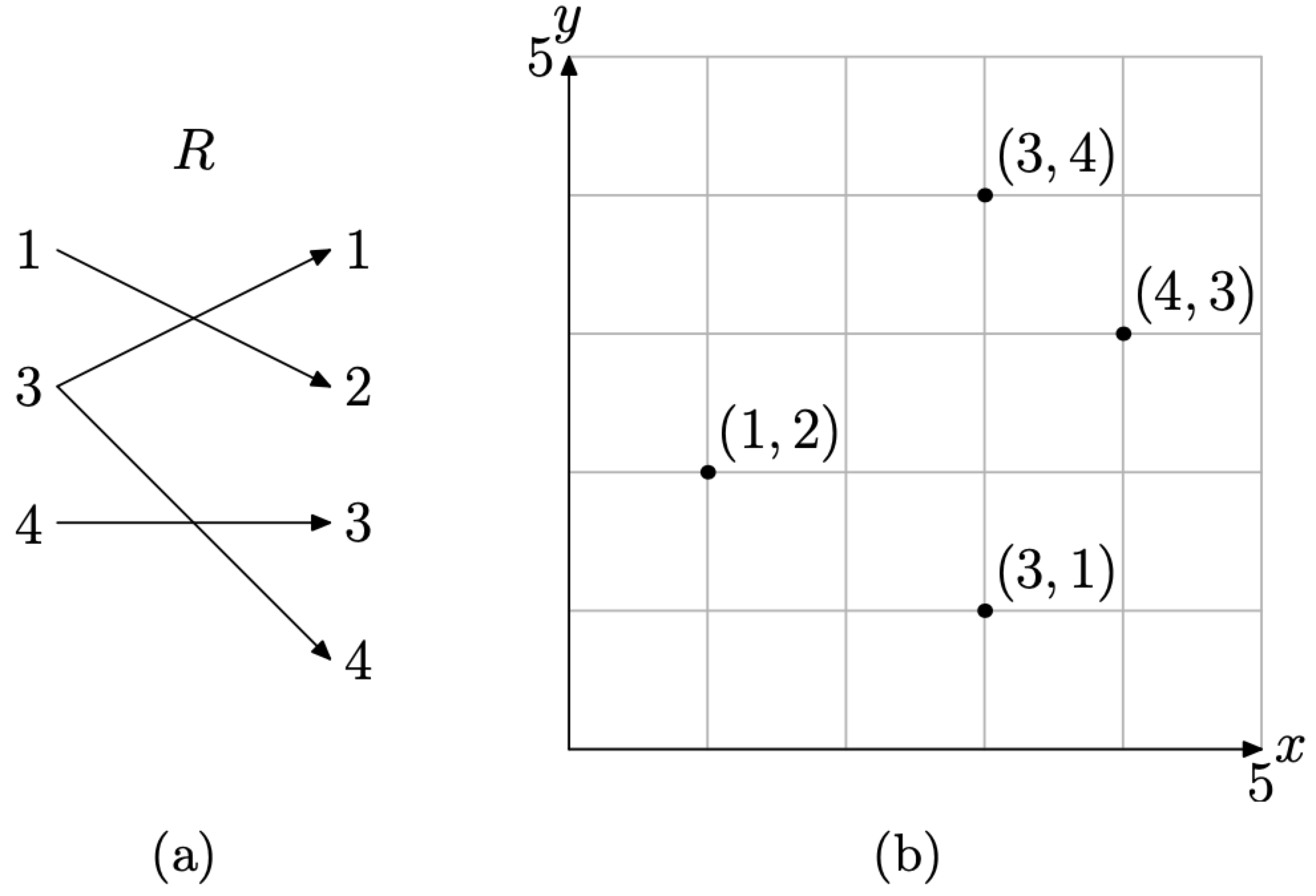
Figure \(\PageIndex{2}\) A mapping diagram and its graph.
In Figure \(\PageIndex{2}\)(a), we’ve created a mapping diagram of the ordered pairs. Note that the domain object 3 is paired with two range elements, namely 1 and 4. Hence the relation R is not a function. It is interesting to note that there are two points in the graph of R in Figure \(\PageIndex{2}\)(b) that have the same first coordinate, namely (3, 1) and (3, 4). This is a signal that the graph of the relation R is not a function. In the next section we will discuss the Vertical Line Test, which will use this dual use of the first coordinate to determine when a relation is a not a function.
Creating the Graph of a Function
Some texts will speak of the graph of an equation, such as “Draw the graph of the equation \(y=x^{2}\).” This instruction raises a number of difficulties.
- First, the instruction provides no direction to the reader; that is, what does the instruction mean? It’s not very helpful.
- Secondly, the instruction is incorrect. You don’t draw the graphs of equations. Rather, you draw the graphs of relations and/or functions. A graph is just another way of representing a function, a relation that pairs each element in its domain with exactly one element in its range.
So, what is the proper instruction? First, we will provide the formal definition of the graph of a function, then we will break it down by means of examples.
The graph of a function is the collection of all ordered pairs of the function. These are usually represented as points in a Cartesian coordinate system.
As an example, consider the function
\[f=\{(1,2),(2,4),(3,1),(4,3)\} \nonumber \]
Readers will note that each object in the domain is paired with one and only one object in the range, as seen in the mapping diagram of Figure \(\PageIndex{3}\)(a).
Thus, we have two representations of the function f, the collection of ordered pairs (3), and the mapping diagram of in Figure \(\PageIndex{3}\)(a). A third representation of the function f is the graph of the ordered pairs of the function, shown in the Cartesian plane in Figure \(\PageIndex{3}\)(b).
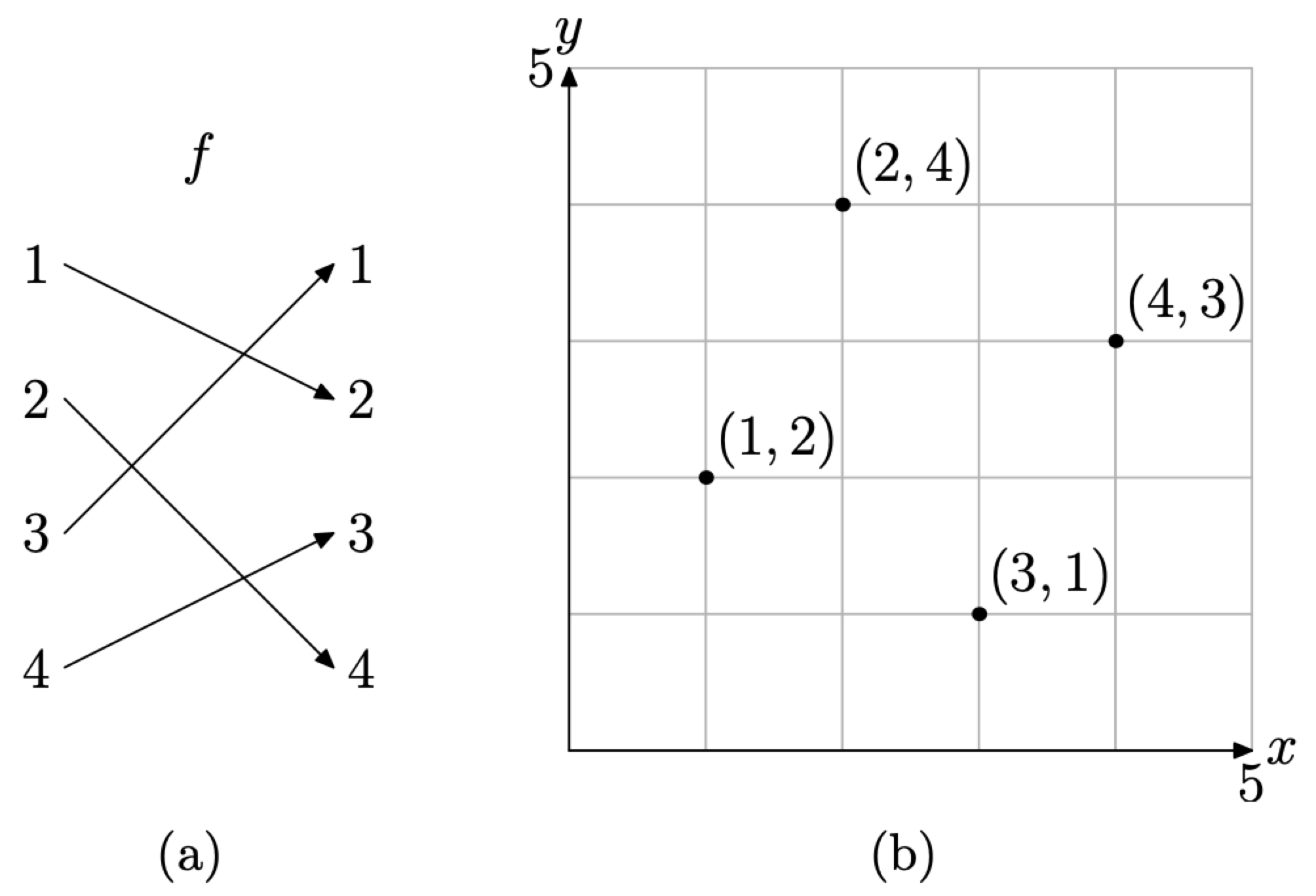
Figure \(\PageIndex{3}\) A mapping diagram and its graph.
When the function is represented by an equation or formula, then we adjust our definition of its graph somewhat.
The graph of f is the set of all ordered pairs \((x, f(x))\) so that x is in the domain of f. In symbols,
\[\text {Graph of } f=\{(x, f(x)) : x \text { is in the domain of } f .\} \nonumber \]
This last definition is most easily explained by example. So, let’s define a function f that maps any real number x to the real number \(x^{2}\); that is, let \(f(x)=x^{2}\). Now, according to Definition, the graph of f is the set of all points \((x, f(x))\), such that x is in the domain of f.
The way is now clear. We begin by creating a table of points \((x, f(x))\), where x is in the domain of the function f defined by \(f(x) = x^{2}\). The choice of x is both subjective and experimental, so we begin by choosing integer values of x between −3 and 3. We then evaluate the function at each of these x-values (e.g., \(f(-3)=(-3)^{2}=9\)). The results are shown in the table in Figure \(\PageIndex{4}\)(a). We then plot the points in our table in the Cartesian plane as shown in Figure \(\PageIndex{4}\)(b).
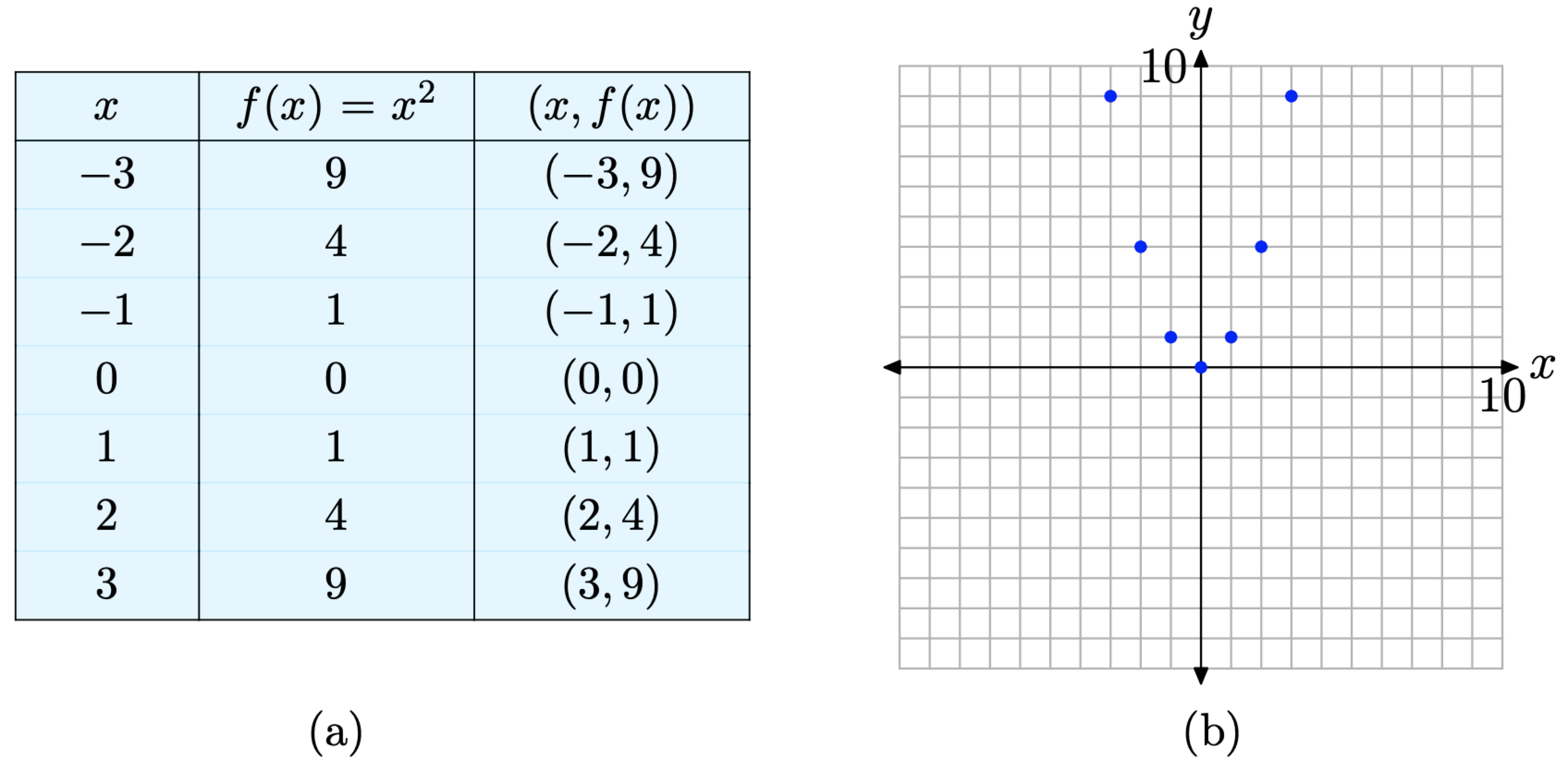
Figure \(\PageIndex{4}\). Plotting pairs satisfying the functional relationship defined by the equation \(f(x)=x^{2}\).
Although this is a good start, the graph in Figure \(\PageIndex{4}\)(b) is far from complete. Definition requires that we plot the ordered pairs \((x, f(x))\) for every value of x that is in the domain of f. We’ve only plotted seven such points, so we’re not done. Let’s add more points to the graph of f. We’ll evaluate the function at each of the x-values shown in the table in Figure \(\PageIndex{5}\)(a), then plot the additional pairs \((x, f(x))\) from the table in the Cartesian plane, as shown in Figure \(\PageIndex{5}\)(b).
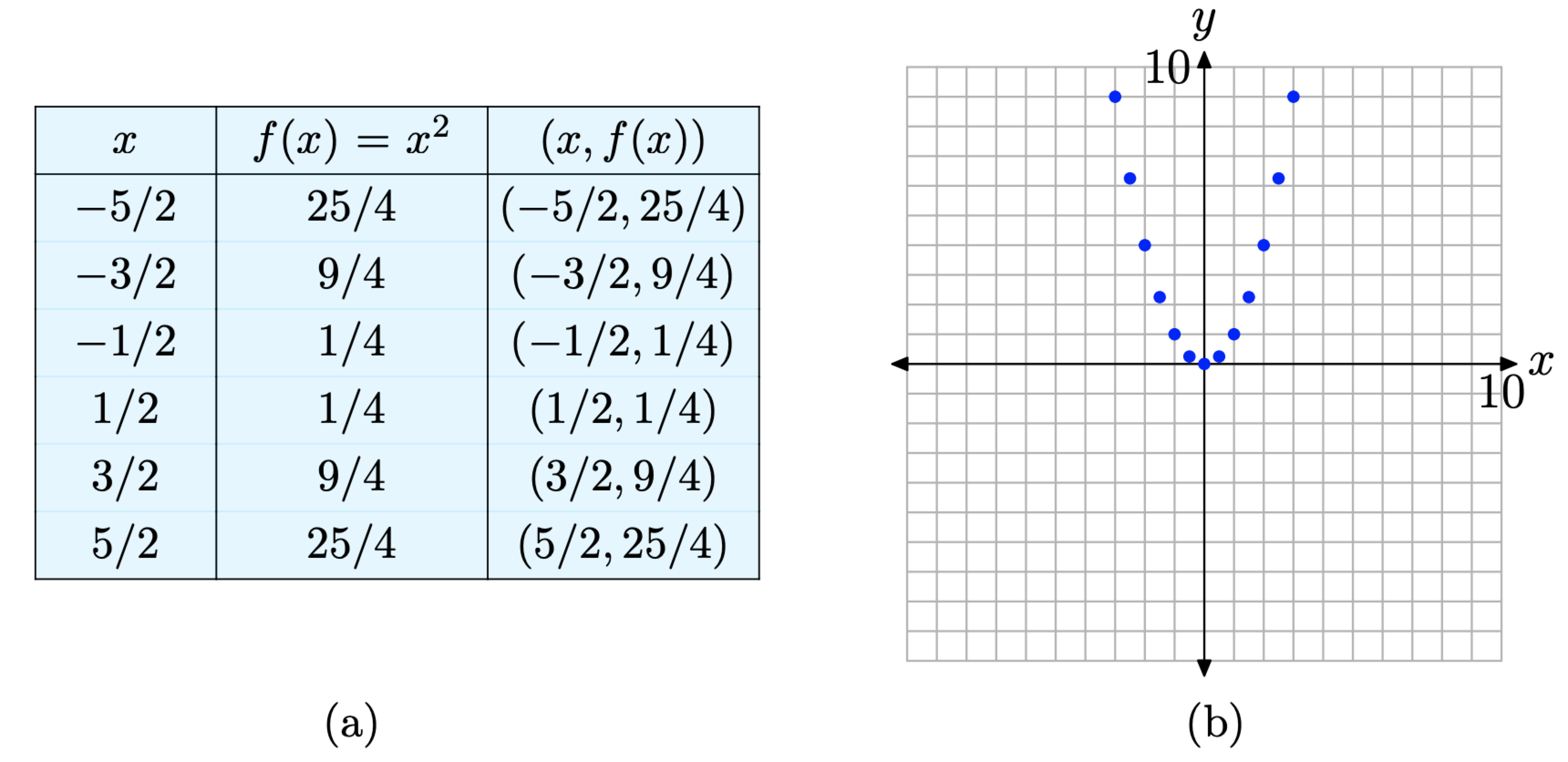
Figure \(\PageIndex{5}\). Plotting additional pairs \((x, f(x))\) defined by the equation \(f(x) = x^{2}\).
We’re still not finished, because we’ve only plotted 13 pairs \((x, f(x))\), such that \(f(x) = x^{2}\). Definition 4 requires that we plot the ordered pairs \((x, f(x))\) for every value of x in the domain of f.
However, a pattern is certainly establishing itself, as seen in Figure \(\PageIndex{5}\)(b). At some point, we need to “make a leap of faith,” and plot all ordered pairs \((x, f(x))\), such that x is in the domain of f. This is done in Figure \(\PageIndex{6}\).
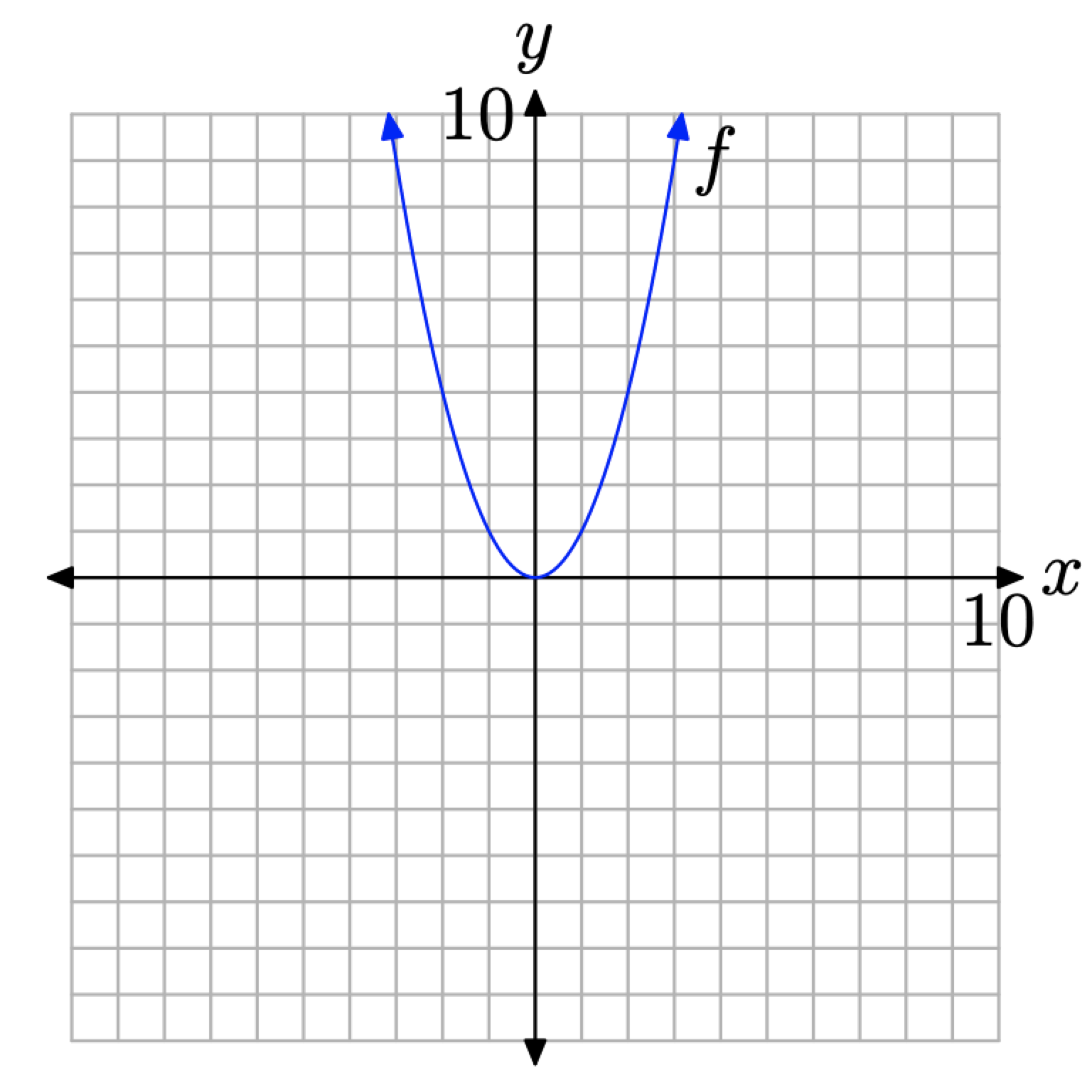
Figure \(\PageIndex{6}\). Plotting all pairs \((x, f(x))\) so that x is in the domain of f.
There are several important points we need to make about the final result in Figure \(\PageIndex{6}\).
- When we draw a smooth curve, such as that shown in Figure \(\PageIndex{6}\), it is important to understand that this is a simply a shortcut for plotting all pairs (x, f(x)), where \(f(x) = x^{2}\) and x is in the domain of f.
- It is important to understand that we are NOT “connecting the dots,” neither with a ruler nor with curved segments. Rather, the curve in Figure \(\PageIndex{6}\) is the result of plotting all of the individual pairs \((x, f(x))\).
- The “arrows” at each end of the curve have an important meaning. Much as the ellipsis at the end of the progression \(2,4,6, \dots\) mean “et-cetera,” the arrows at each end of the curve have a similar meaning. The arrow at the end of the left-half of the curve indicates that the graph continues opening upward and to the left, while the arrow at the end of the right-half of the curve indicates that the graph continues opening upward and to the right.
Creating Graphs by Hand
We’re going to look at several basic graphs, which we’ll create by employing the strategy used to create the graph of \(f(x) = x^{2}\). First, let’s summarize that process.
If a function is defined by an equation, you can create the graph of the function as follows.
- Select several values of x in the domain of the function f.
- Use the selected values of x to create a table of pairs (x, f(x)) that satisfy the equation that defines the function f.
- Create a Cartesian coordinate system on a sheet of graph paper. Label and scale each axis, then plot the pairs (x, f(x)) from your table on your coordinate system.
- If the plotted pairs (x, f(x)) provide enough of a pattern for you to intuit the shape of the graph of f, make the “leap of faith” and plot all pairs that satisfy the equation defining f by drawing a smooth curve on your coordinate system. Of course, this curve should contain all previously plotted pairs.
- If your plotted pairs do not provide enough of a pattern to determine the final shape of the graph of f, then add more pairs to your table and plot them on your Cartesian coordinate system. Continue in this manner until you are confident in the shape of the graph of f.
Let’s look at an example.
Sketch the graph of the function defined by the equation \(f(x)=x^{3}\).
Solution
We’ll start with x-values \(-2,-1,0,1,\) and 2, then use the equation \(f(x)=x^{3}\) to determine pairs (x, f(x)) (e.g., \(f(-2)=(-2)^{3}=-8\)). These are listed in the table in Figure \(\PageIndex{7}\)(a). We then plot the points from the table on a Cartesian coordinate system, as shown in Figure \(\PageIndex{7}\)(b).
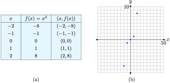
Figure \(\PageIndex{7}\). Plotting pairs (x, f(x)) defined by the equation \(f(x)=x^{3}\).
We’re a bit unsure of the shape of the graph of f, so we’ll add a few more pairs to our table and plot them. This is shown in Figures \(\PageIndex{8}\)(a) and (b).
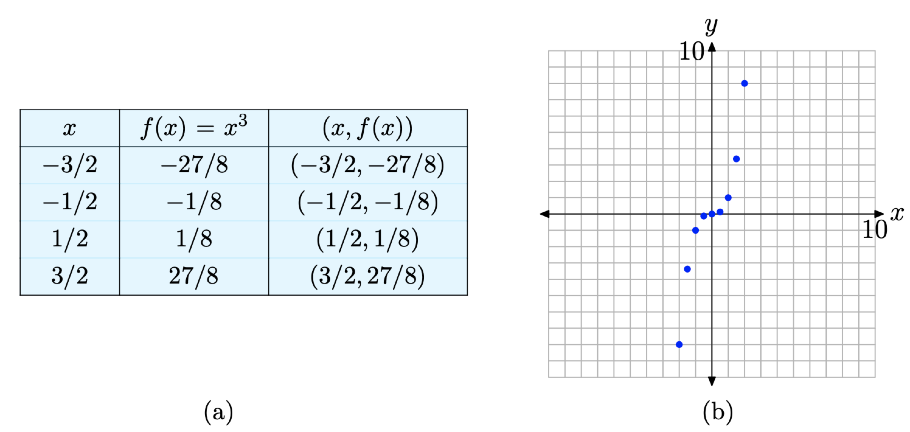
Figure \(\PageIndex{8}\). Plotting additional pairs (x, f(x)) defined by the equation \(f(x)=x^{3}\).
The additional pairs fill in the shape of f in Figure \(\PageIndex{8}\)(b) a bit better than those in Figure \(\PageIndex{7}\)(b), enough so that we’re confident enough to make a “leap of faith” and draw the final shape of the graph of \(f(x)=x^{3}\) in Figure \(\PageIndex{9}\).
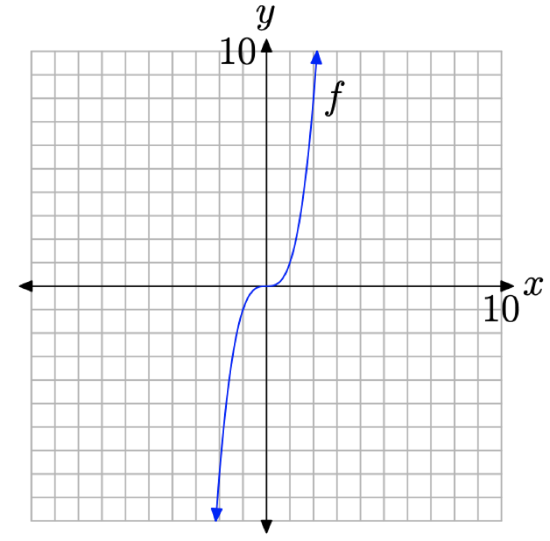
Figure \(\PageIndex{9}\). The final graph of \(f(x)=x^{3}\).
Let’s look at another example.
Sketch the graph of \(f(x)=\sqrt{x}\)
Solution
Again, we’ll start by selecting several values of x in the domain of f. In this case, \(f(x)=\sqrt{x}\), and it’s not possible to take the square root of a negative number. Also, if we’re creating a table of pairs by hand, it’s good strategy to select known squares. Thus, we’ll use x = 0, 1, 4, and 9 for starters.
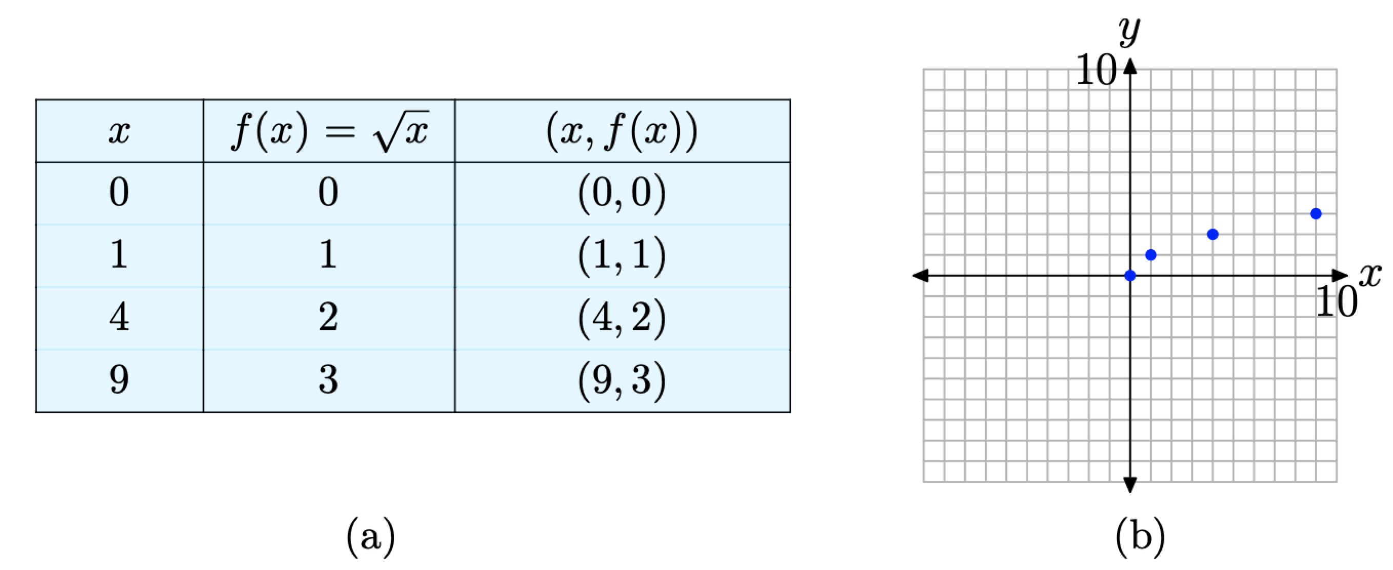
Figure \(\PageIndex{10}\). Plotting pairs (x, f(x)) defined by the equation \(f(x)=\sqrt{x}\).
Some might be ready to make a “leap of faith” based on these initial results. Others might want to use a calculator to compute decimal approximations for additional square roots. The resulting pairs are shown in the table in Figure \(\PageIndex{11}\)(a) and the additional pairs are plotted in Figure \(\PageIndex{11}\)(b).
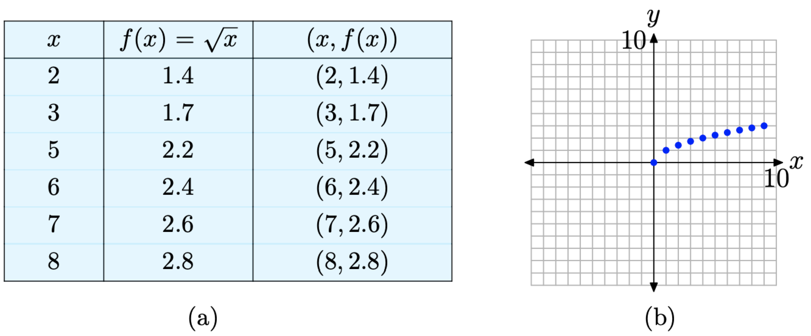
Figure \(\PageIndex{11}\) Plotting additional pairs (x, f(x)) defined by the equation \(f(x)=\sqrt{x}\)
The pattern in Figure \(\PageIndex{11}\)(b) is clear enough to make a “leap of faith” and complete the graph as shown in Figure \(\PageIndex{12}\).
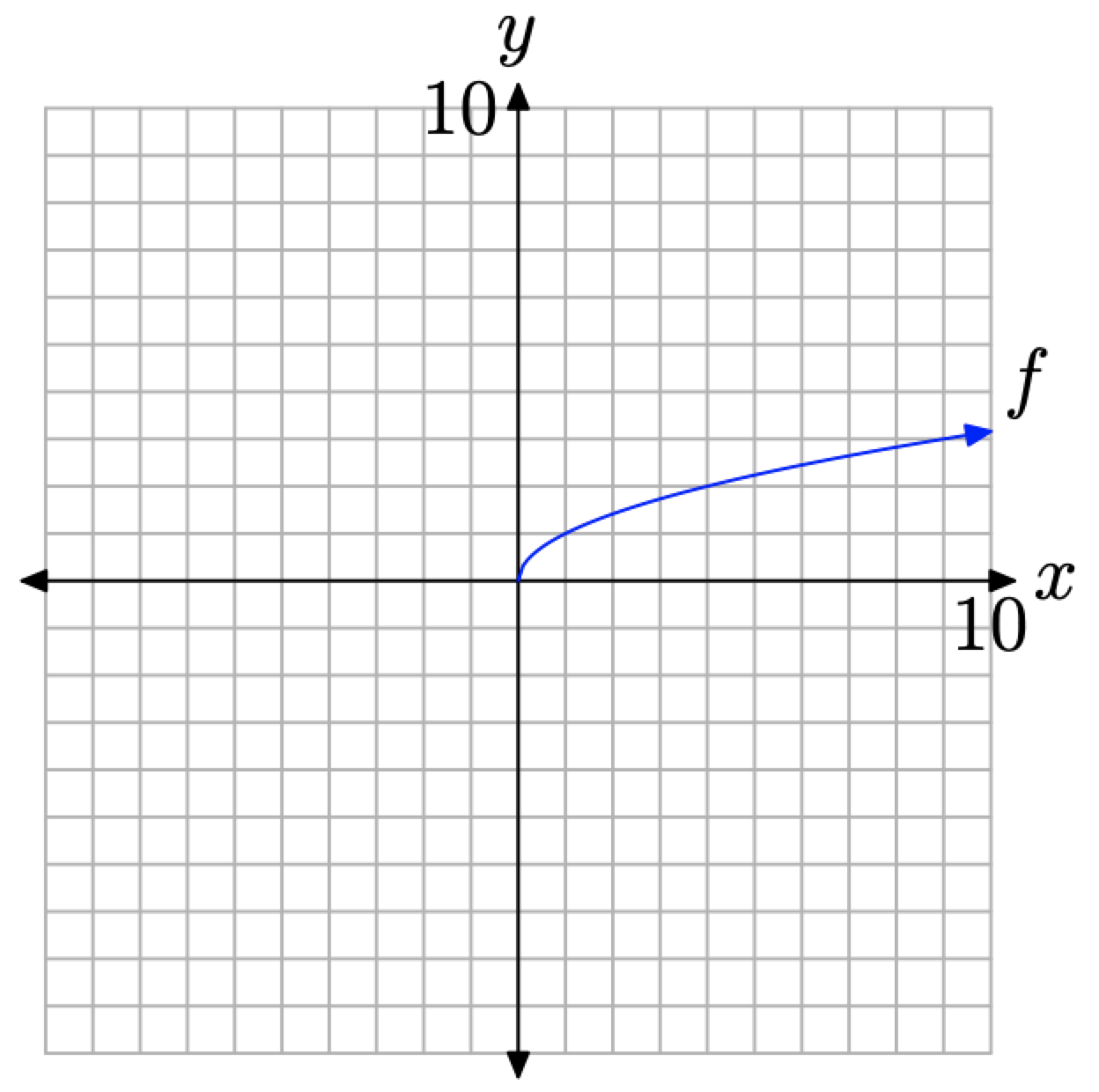
Figure \(\PageIndex{12}\). The graph of f defined by the equation \(f(x)=\sqrt{x}\).
Using the Table Feature of the Graphing Calculator
The TABLE feature on your graphing calculator can be of immense help when creating tables of points that satisfy the equation defining the function f. Let’s look at an example
Sketch the graph of \(f(x)=|x|\)
Solution
Enter the function \(f(x)=|x|\) in the \(\mathrm{Y}=\) menu as follows.
- Press the Y= button on your calculator. This will open the Y= menu as shown in Figure \(\PageIndex{13}\)(a). Use the arrow keys and the CLEAR button on your calculator to delete any existing functions.
- Press the MATH button to open the menu shown in Figure \(\PageIndex{13}\)(b).
- Press the right-arrow on your calculator to select the NUM submenu as shown in Figure \(\PageIndex{13}\)(c).
- Select 1:abs(, then enter X and close the parentheses, as shown in Figure \(\PageIndex{13}\)(d).
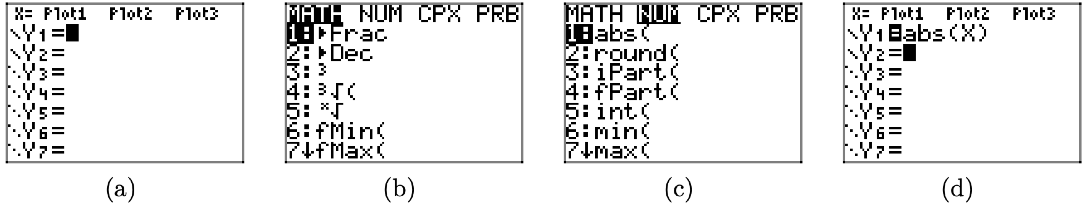
Figure \(\PageIndex{13}\). Entering \(f(x)=|x|\) in the \(\mathrm{Y}=\) menu.
We will now use the TABLE feature of the graphing calculator to help create a table of pairs (x, f(x)) satisfying the equation \(f(x) = |x|\). Proceed as follows.
- Select 2nd TBLSET (i.e., push the 2nd button followed by TBLSET), which is located over the WINDOW button. Enter TblStart=-3, \(\Delta \mathrm{Tb} 1=1\), and set the independent and dependent variables to Auto (this is done by highlighting Auto and pressing the Enter button), as shown in Figure \(\PageIndex{14}\)(a).
- Press 2nd TABLE, which is located above the GRAPH button, to produce the table of pairs (x, f(x)) shown in Figure \(\PageIndex{14}\)(b).
We’ve plotted the pairs directly from the calculator onto a Cartesian coordinate system on graph paper in Figure \(\PageIndex{14}\)(c).
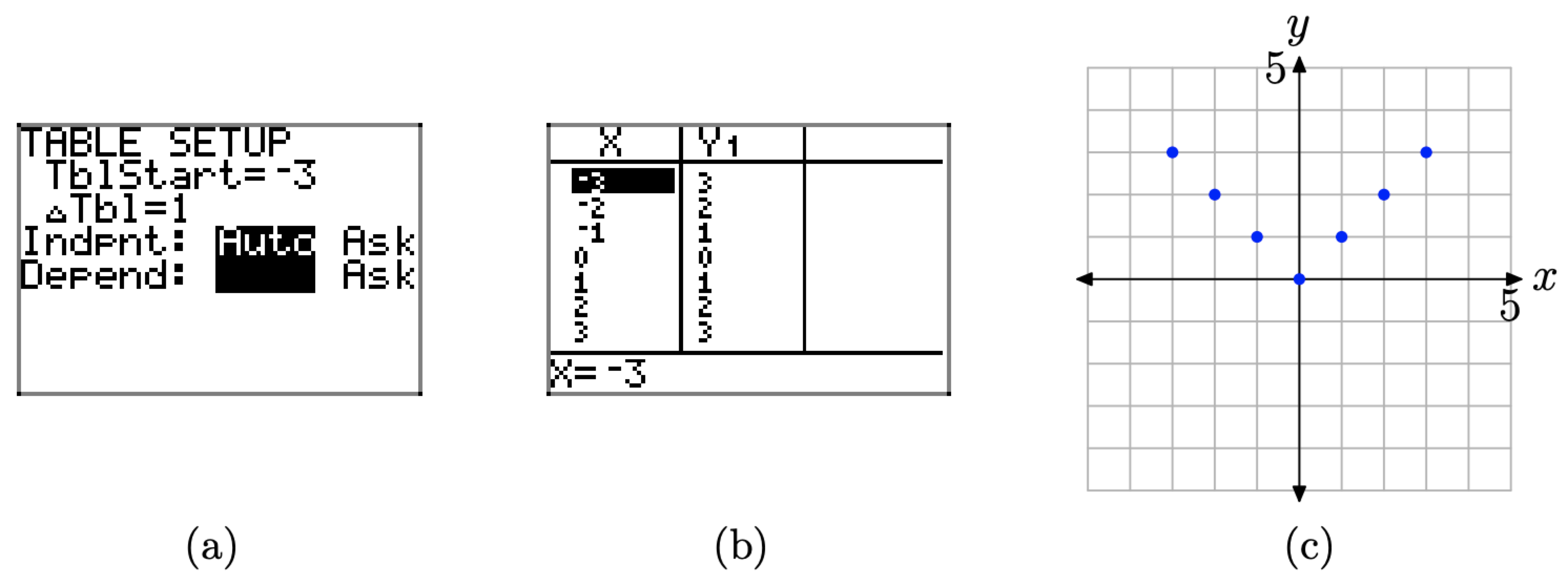
Figure \(\PageIndex{14}\). Creating a table with the TABLE feature of the graphing calculator.
Based on what we see in Figure \(\PageIndex{14}\)(c), we’re ready to make a “leap of faith” and draw the graph of f shown in Figure \(\PageIndex{15}\).
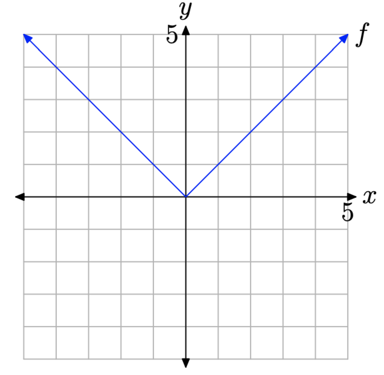
Figure \(\PageIndex{15}\). The graph of f defined by \(f(x) = |x|\).
Alternatively, or as a check, we can have the graphing calculator draw the graph for us. Push the ZOOM button, then select 6:ZStandard (shown in Figure \(\PageIndex{16}\)(a)) to produce the graph shown in Figure \(\PageIndex{16}\)(b).
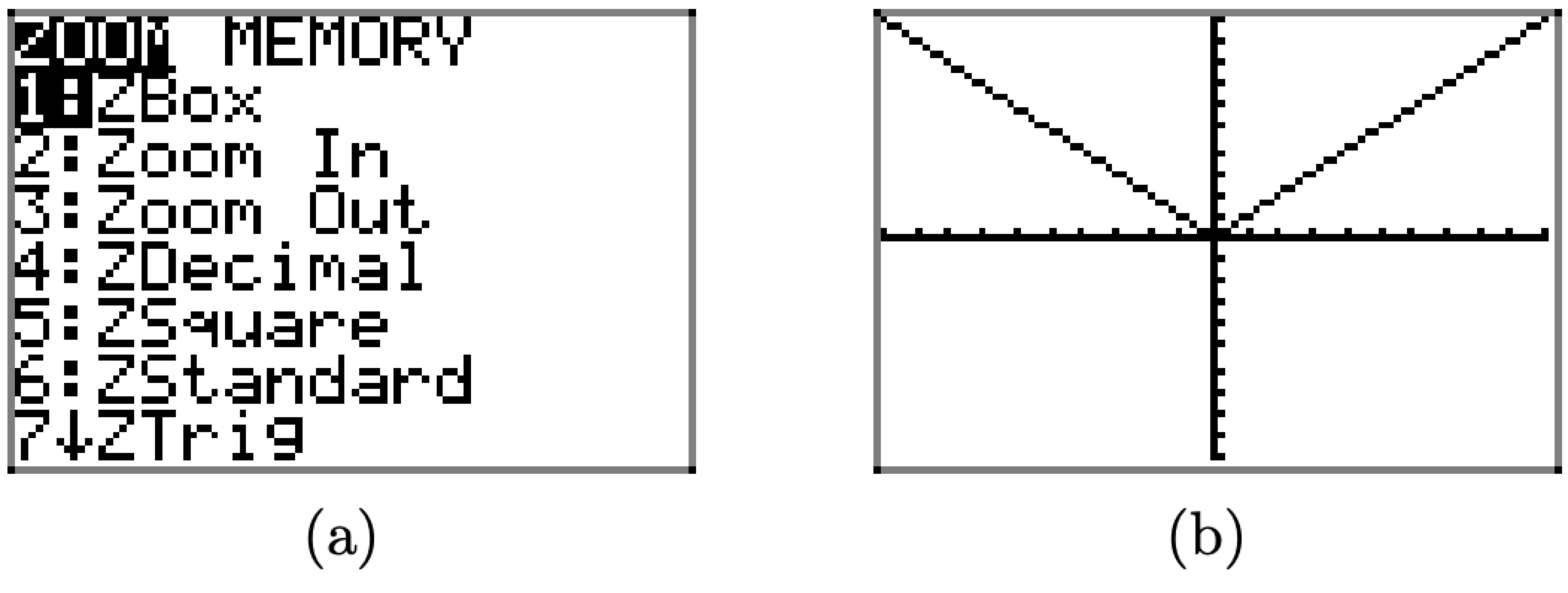
Figure \(\PageIndex{16}\). Creating the graph of \(f(x) = |x|\) with the graphing calculator.
Adjusting the Viewing Window
In Example \(\PageIndex{3}\), we used the graphing calculator to draw the graph of the function defined by the equation \(f(x) = |x|\). For the functions we’ve encountered thus far, drawing their graphs using the graphing calculator is pretty trivial. Simply enter the equation in the Y= menu, then press the ZOOM button and select 6:ZStandard. However, if the graph of a function doesn’t fit (or even appear) in the “standard” viewing window, it can be quite challenging to find optimal view settings so that the important features of the graph are visible.
Indeed, as one might not even know what “important” features to look for, setting the viewing window is usually highly subjective and experimental by nature. Let’s look at some examples.
Use a graphing calculator to sketch the graph of \(f(x)=56-x-x^{2}\). Experiment with the WINDOW settings until you feel you have a viewing window that exhibits the important features of the graph.
Solution
First, start by entering the function in the Y= menu, as shown in Figure \(\PageIndex{17}\)(a). The caret ˆon the keyboard is used for exponents. Press the ZOOM button and select 6:ZStandard to produce the graph shown in Figure \(\PageIndex{17}\)(b).
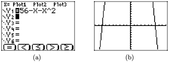
Figure \(\PageIndex{17}\). The graph of \(f(x)=56-x-x^{2}\) in the “standard” viewing window.
As the graph draws, observe that the graph rises from the bottom of the screen, leaves the top of the screen, then returns, falling from the top of the screen and leaving again at the bottom of the screen. This would indicate that there must be some sort of “turning point” that is not visible at the top of the screen.
Press the WINDOW button to reveal the “standard viewing window” settings shown in Figure \(\PageIndex{18}\)(a). The following legend explains each of the WINDOW parameters in Figure \(\PageIndex{18}\)(a).
\(\begin{array} { lll} Xmin & =& x-value of left edge of viewing window \\
Xmax &=& x-value of right edge of viewing window \\
Xscl &=& x-axis tick increment \\
Y min &=& y-value of bottom edge of viewing window \\
Y max &=& y-value of top edge of viewing window \\
Y scl &=& y-axis tick increment \end{array}\)
It is easy to evaluate the function \(f(x)=56-x-x^{2}\) at \(x = 0\). Indeed, \(f(0) = 56−0−0^2 = 56\). This indicates that the graph of f must pass through the point (0, 56). This gives us a clue at how we should set the upper bound on our viewing window. Set Ymax = 60, as shown in Figure \(\PageIndex{18}\)(b), then press the GRAPH button to produce the graph and viewing window shown in Figure \(\PageIndex{18}\)(c).
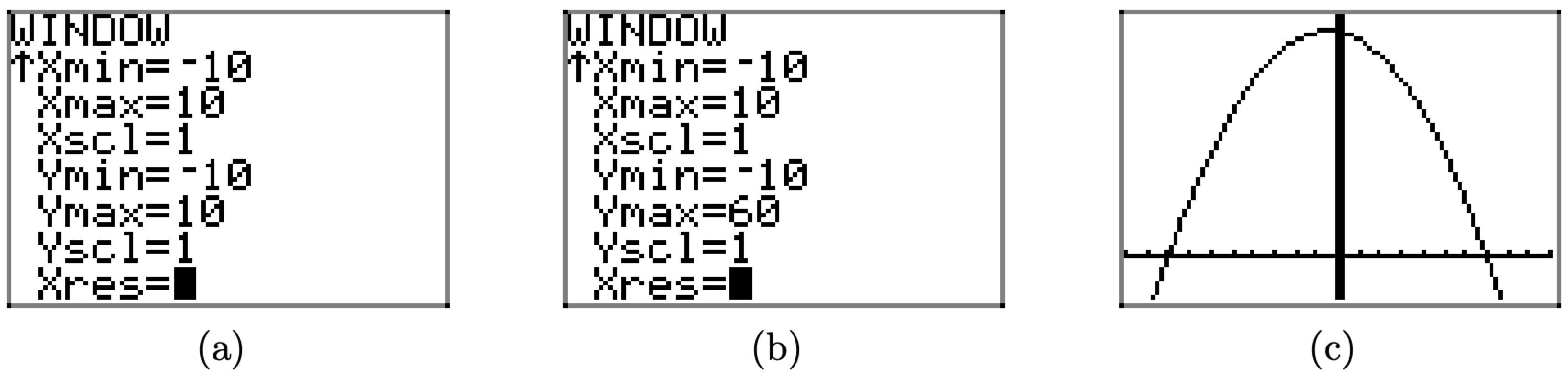
Figure \(\PageIndex{18}\). Changing the viewing window.
Although the viewing window in Figure \(\PageIndex{18}\)(c) shows the “turning point” of the graph of f, we will make some additional changes to the window settings, as shown in Figure \(\PageIndex{19}\)(a). First, we “widen” the viewing window a bit, setting Xmin = -15 and Xmax = 15, then we set tick marks on the x-axis every 5 units with Xscl = 5. Next, to create a little room at the top of the screen, we set Ymax = 100, then we “balance” this setting with Ymin = -100. Finally, we set tick marks on the y-axis every 10 units with Yscl = 10.
Push the GRAPH button to view the effects of these changes to the WINDOW parameters in Figure \(\PageIndex{19}\)(b). Note that these settings are highly subjective, and what one reader might find quite pleasing will not necessarily find favor with other readers.
However, what is important is the fact that we’ve captured the “important features” of the graph of \(f(x)=56-x-x^{2}\). Note that this is a very controversial statement. If one is just beginning to learn about the graphs of functions, how is one to determine what are the “important features” of the graph? Unfortunately, the answer to this question is, “through experience.” Undoubtedly, this is a very frustrating phrase for readers to hear, but at least it’s truthful. The more graphs that you draw, the more you will learn how to look for “turning points,” “end-behavior,” “x- and y-intercepts,” and the like.
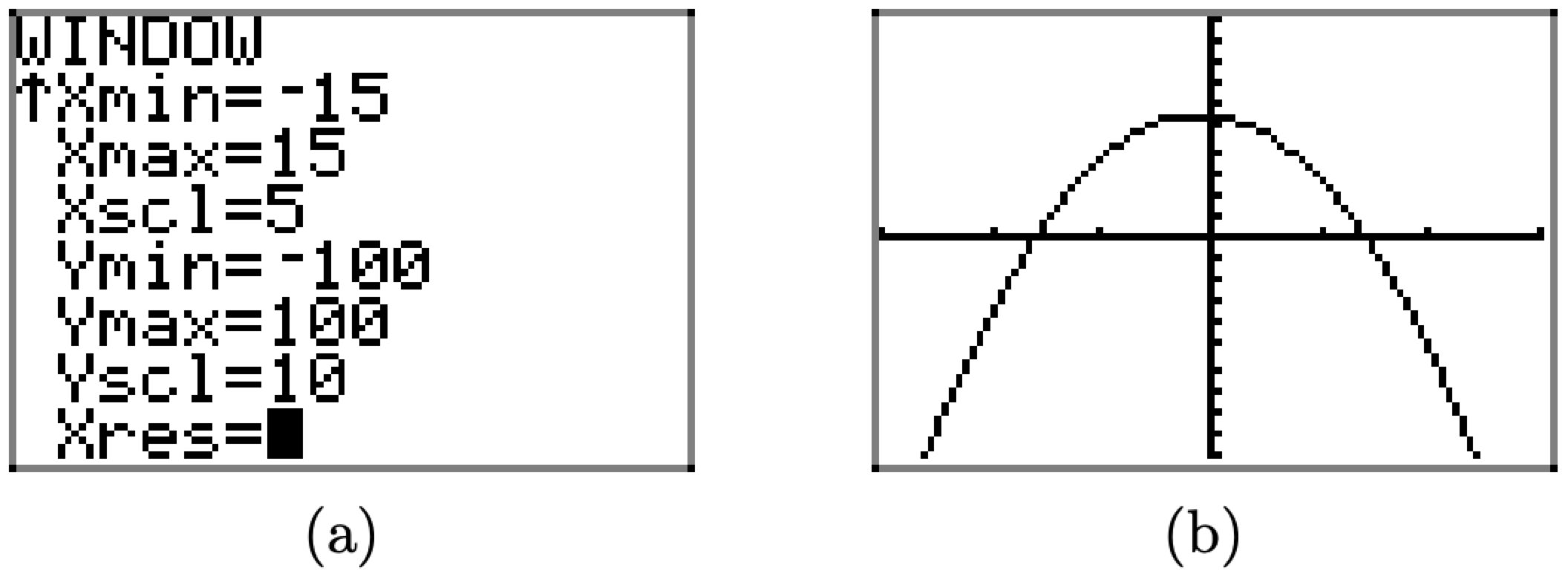
Figure \(\PageIndex{19}\). Improving the WINDOW settings.
For example, how do we know that the WINDOW settings in Figure \(\PageIndex{19}\)(a) determine a viewing window (Figure \(\PageIndex{19}\)(b)) that reveals all “important features” of the graph? The answer at this point is, “we don’t, not without further experiment.” For example, the careful reader might want to try the window settings Xmin=-50, Xmax=50, Xscl=10, Ymin=-500, Ymax=500, and Yscl=100 to see if any unexpected behavior crops up.
Let’s look at one last example.
Sketch the graph of the function f defined by the equation \(f(x) = x^{4}+9 x^{3}-117 x^{2}-265 x+2100\).
Solution
Load the function into the Y= menu (shown in Figure \(\PageIndex{20}\)(a)) and select 6:ZStandard to produce the graph shown in Figure \(\PageIndex{20}\)(b).
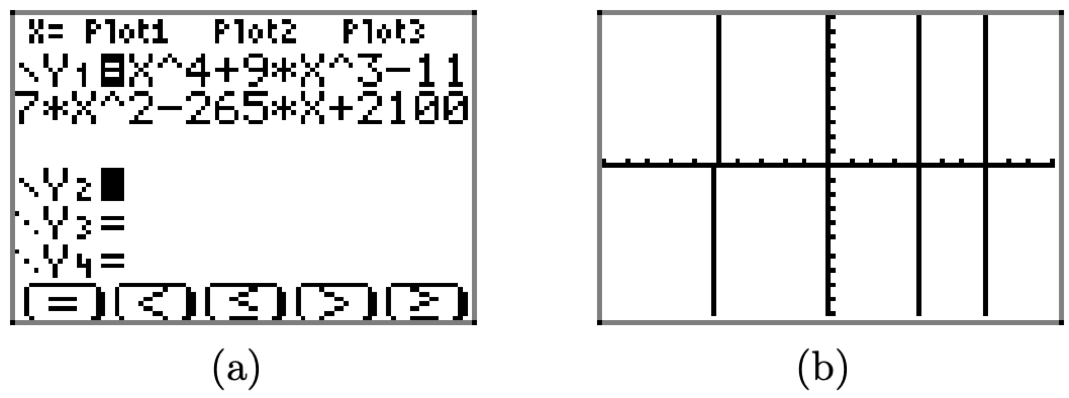
Figure \(\PageIndex{20}\) Sketching the graph of \(f(x) = x^{4}+9 x^{3}-117 x^{2}-265 x+2100\).
As the graph draws, observe that it rises form the bottom of the viewing window, leaves the top of the viewing window, then returns to fall off the bottom of the viewing window, then returns again and rises off the top of the viewing window.
We notice that f(0) = 2100, so we’ll need to set the top of the viewing window to that value or higher. With this thought in mind, we’ll set Ymax=3000, then set Ymin=-3000 for balance, then to avoid a million little tick marks, we’ll set Yscl=1000, all shown in Figure \(\PageIndex{21}\)(a). Pressing the GRAPH button then produces the image shown in Figure \(\PageIndex{21}\)(b).
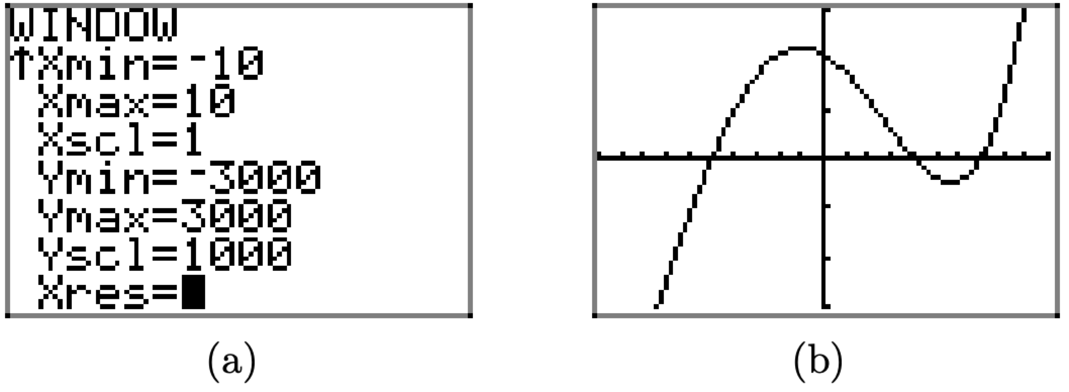
Figure \(\PageIndex{21}\) Adjusting the viewing window.
Does it appear that we have all of the “important features” of this graph displayed in our viewing window? Note that we did not experiment very much. Perhaps we should try expanding the window a bit more to see if we have missed any important behavior. With that thought in mind, we set Xmin=-20, Xmax=20, and to avoid a ton of tick marks, Xscl=5, as shown in Figure \(\PageIndex{22}\)(a). Pushing the GRAPH button produces the image in Figure \(\PageIndex{22}\)(b).
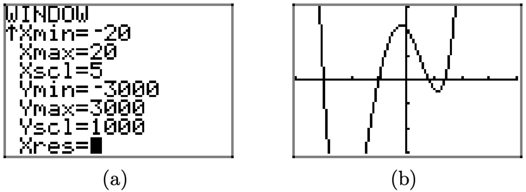
Figure \(\PageIndex{22}\) Adjusting the viewing window again reveals behavior not seen.
Note that the viewing window in Figure \(\PageIndex{22}\)(b) reveals behavior not seen in the viewing window of Figure \(\PageIndex{21}\)(b). If we had not experimented further, if we had not expanded the viewing window, we would not have seen this new behavior. This is an important lesson.
Note that one of the “turning points” of the graph in Figure \(\PageIndex{22}\)(b) lies off the bottom of the viewing window. We’ll make one more adjustment to include this important feature. Set Ymin=-10000, Ymax=10000, and Yscl=5000, as shown in Figure \(\PageIndex{23}\)(a), then push the GRAPH button to produce the image shown in Figure \(\PageIndex{23}\)(b).
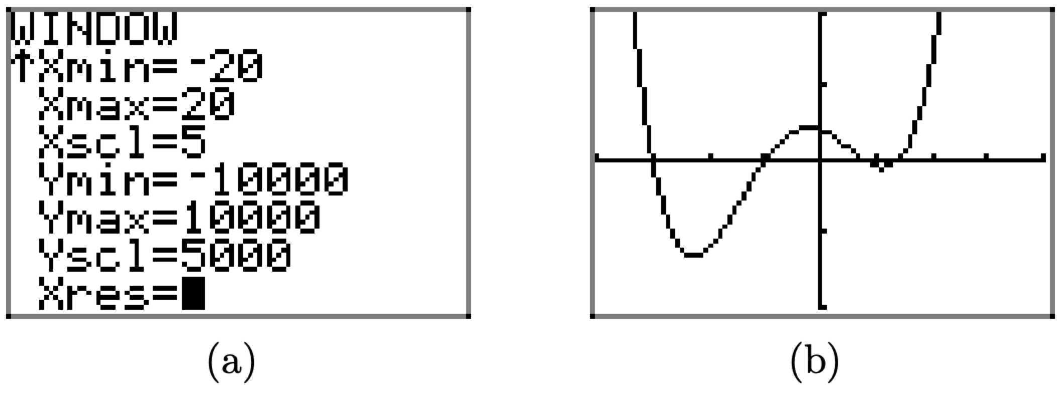
Figure \(\PageIndex{23}\). Adjusting the viewing window again reveals behavior not seen.
The graph in Figure \(\PageIndex{23}\)(b) shows all of the “important features” of the graph of f, but the careful reader will continue to experiment, expanding the viewing window to ascertain the truth of this statement.