
2.1: Introduction to Functions
- Page ID
- 19685

\( \newcommand{\vecs}[1]{\overset { \scriptstyle \rightharpoonup} {\mathbf{#1}} } \)
\( \newcommand{\vecd}[1]{\overset{-\!-\!\rightharpoonup}{\vphantom{a}\smash {#1}}} \)
\( \newcommand{\dsum}{\displaystyle\sum\limits} \)
\( \newcommand{\dint}{\displaystyle\int\limits} \)
\( \newcommand{\dlim}{\displaystyle\lim\limits} \)
\( \newcommand{\id}{\mathrm{id}}\) \( \newcommand{\Span}{\mathrm{span}}\)
( \newcommand{\kernel}{\mathrm{null}\,}\) \( \newcommand{\range}{\mathrm{range}\,}\)
\( \newcommand{\RealPart}{\mathrm{Re}}\) \( \newcommand{\ImaginaryPart}{\mathrm{Im}}\)
\( \newcommand{\Argument}{\mathrm{Arg}}\) \( \newcommand{\norm}[1]{\| #1 \|}\)
\( \newcommand{\inner}[2]{\langle #1, #2 \rangle}\)
\( \newcommand{\Span}{\mathrm{span}}\)
\( \newcommand{\id}{\mathrm{id}}\)
\( \newcommand{\Span}{\mathrm{span}}\)
\( \newcommand{\kernel}{\mathrm{null}\,}\)
\( \newcommand{\range}{\mathrm{range}\,}\)
\( \newcommand{\RealPart}{\mathrm{Re}}\)
\( \newcommand{\ImaginaryPart}{\mathrm{Im}}\)
\( \newcommand{\Argument}{\mathrm{Arg}}\)
\( \newcommand{\norm}[1]{\| #1 \|}\)
\( \newcommand{\inner}[2]{\langle #1, #2 \rangle}\)
\( \newcommand{\Span}{\mathrm{span}}\) \( \newcommand{\AA}{\unicode[.8,0]{x212B}}\)
\( \newcommand{\vectorA}[1]{\vec{#1}} % arrow\)
\( \newcommand{\vectorAt}[1]{\vec{\text{#1}}} % arrow\)
\( \newcommand{\vectorB}[1]{\overset { \scriptstyle \rightharpoonup} {\mathbf{#1}} } \)
\( \newcommand{\vectorC}[1]{\textbf{#1}} \)
\( \newcommand{\vectorD}[1]{\overrightarrow{#1}} \)
\( \newcommand{\vectorDt}[1]{\overrightarrow{\text{#1}}} \)
\( \newcommand{\vectE}[1]{\overset{-\!-\!\rightharpoonup}{\vphantom{a}\smash{\mathbf {#1}}}} \)
\( \newcommand{\vecs}[1]{\overset { \scriptstyle \rightharpoonup} {\mathbf{#1}} } \)
\(\newcommand{\longvect}{\overrightarrow}\)
\( \newcommand{\vecd}[1]{\overset{-\!-\!\rightharpoonup}{\vphantom{a}\smash {#1}}} \)
\(\newcommand{\avec}{\mathbf a}\) \(\newcommand{\bvec}{\mathbf b}\) \(\newcommand{\cvec}{\mathbf c}\) \(\newcommand{\dvec}{\mathbf d}\) \(\newcommand{\dtil}{\widetilde{\mathbf d}}\) \(\newcommand{\evec}{\mathbf e}\) \(\newcommand{\fvec}{\mathbf f}\) \(\newcommand{\nvec}{\mathbf n}\) \(\newcommand{\pvec}{\mathbf p}\) \(\newcommand{\qvec}{\mathbf q}\) \(\newcommand{\svec}{\mathbf s}\) \(\newcommand{\tvec}{\mathbf t}\) \(\newcommand{\uvec}{\mathbf u}\) \(\newcommand{\vvec}{\mathbf v}\) \(\newcommand{\wvec}{\mathbf w}\) \(\newcommand{\xvec}{\mathbf x}\) \(\newcommand{\yvec}{\mathbf y}\) \(\newcommand{\zvec}{\mathbf z}\) \(\newcommand{\rvec}{\mathbf r}\) \(\newcommand{\mvec}{\mathbf m}\) \(\newcommand{\zerovec}{\mathbf 0}\) \(\newcommand{\onevec}{\mathbf 1}\) \(\newcommand{\real}{\mathbb R}\) \(\newcommand{\twovec}[2]{\left[\begin{array}{r}#1 \\ #2 \end{array}\right]}\) \(\newcommand{\ctwovec}[2]{\left[\begin{array}{c}#1 \\ #2 \end{array}\right]}\) \(\newcommand{\threevec}[3]{\left[\begin{array}{r}#1 \\ #2 \\ #3 \end{array}\right]}\) \(\newcommand{\cthreevec}[3]{\left[\begin{array}{c}#1 \\ #2 \\ #3 \end{array}\right]}\) \(\newcommand{\fourvec}[4]{\left[\begin{array}{r}#1 \\ #2 \\ #3 \\ #4 \end{array}\right]}\) \(\newcommand{\cfourvec}[4]{\left[\begin{array}{c}#1 \\ #2 \\ #3 \\ #4 \end{array}\right]}\) \(\newcommand{\fivevec}[5]{\left[\begin{array}{r}#1 \\ #2 \\ #3 \\ #4 \\ #5 \\ \end{array}\right]}\) \(\newcommand{\cfivevec}[5]{\left[\begin{array}{c}#1 \\ #2 \\ #3 \\ #4 \\ #5 \\ \end{array}\right]}\) \(\newcommand{\mattwo}[4]{\left[\begin{array}{rr}#1 \amp #2 \\ #3 \amp #4 \\ \end{array}\right]}\) \(\newcommand{\laspan}[1]{\text{Span}\{#1\}}\) \(\newcommand{\bcal}{\cal B}\) \(\newcommand{\ccal}{\cal C}\) \(\newcommand{\scal}{\cal S}\) \(\newcommand{\wcal}{\cal W}\) \(\newcommand{\ecal}{\cal E}\) \(\newcommand{\coords}[2]{\left\{#1\right\}_{#2}}\) \(\newcommand{\gray}[1]{\color{gray}{#1}}\) \(\newcommand{\lgray}[1]{\color{lightgray}{#1}}\) \(\newcommand{\rank}{\operatorname{rank}}\) \(\newcommand{\row}{\text{Row}}\) \(\newcommand{\col}{\text{Col}}\) \(\renewcommand{\row}{\text{Row}}\) \(\newcommand{\nul}{\text{Nul}}\) \(\newcommand{\var}{\text{Var}}\) \(\newcommand{\corr}{\text{corr}}\) \(\newcommand{\len}[1]{\left|#1\right|}\) \(\newcommand{\bbar}{\overline{\bvec}}\) \(\newcommand{\bhat}{\widehat{\bvec}}\) \(\newcommand{\bperp}{\bvec^\perp}\) \(\newcommand{\xhat}{\widehat{\xvec}}\) \(\newcommand{\vhat}{\widehat{\vvec}}\) \(\newcommand{\uhat}{\widehat{\uvec}}\) \(\newcommand{\what}{\widehat{\wvec}}\) \(\newcommand{\Sighat}{\widehat{\Sigma}}\) \(\newcommand{\lt}{<}\) \(\newcommand{\gt}{>}\) \(\newcommand{\amp}{&}\) \(\definecolor{fillinmathshade}{gray}{0.9}\)Our development of the function concept is a modern one, but quite quick, particularly in light of the fact that today’s definition took over 300 years to reach its present state. We begin with the definition of a relation.
Relations
We use the notation (2, 4) to denote what is called an ordered pair. If you think of the positions taken by the ordered pairs (4, 2) and (2, 4) in the coordinate plane (see Figure \(\PageIndex{1}\)), then it is immediately apparent why order is important. The ordered pair (4, 2) is simply not the same as the ordered pair (2, 4).
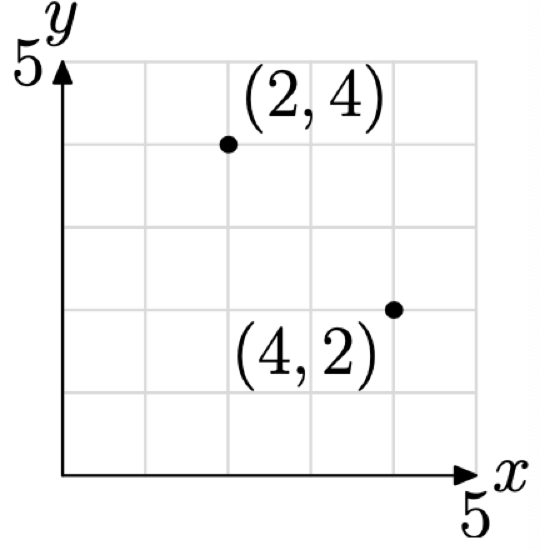
Figure \(\PageIndex{1}\)
The first element of an ordered pair is called its abscissa. The second element of an ordered pair is called its ordinate. Thus, for example, the abscissa of (4, 2) is 4, while the ordinate of (4, 2) is 2.
A collection of ordered pairs is called a relation. (2)
For example, the collection of ordered pairs \[R=\{(0,1),(0,2),(3,4)\} \nonumber \] is a relation.
The domain of a relation is the collection of all abscissas of each ordered pair.
Thus, the domain of the relation R in (2) is \[\text { Domain }=\{0,3\} \nonumber \]
Note that we list each abscissa only once.
The range of a relation is the collection of all ordinates of each ordered pair.
Thus, the range of the relation R in (2) is \[\text { Range }=\{1,2,4\} \nonumber \]
Let’s look at an example.
Consider the relation T defined by \[T=\{(1,2),(3,2),(4,5)\} \nonumber \]
What are the domain and range of this relation?
Solution
The domain is the collection of abscissas of each ordered pair. Hence, the domain of T is \[\text { Domain }=\{1,3,4\} \nonumber \]
The range is the collection of ordinates of each ordered pair. Hence, the range of T is \[\text { Range }=\{2,5\} \nonumber \]
Note that we list each ordinate in the range only once.
In Example \(\PageIndex{1}\), the relation is described by listing the ordered pairs. This is not the only way that one can describe a relation. For example, a graph certainly represents a collection of ordered pairs.
Consider the graph of the relation S shown in Figure \(\PageIndex{2}\).
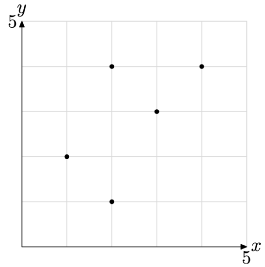
Figure \(\PageIndex{2}\) The graph of a relation.
What are the domain and range of the relation S?
Solution
There are five ordered pairs (points) plotted in Figure \(\PageIndex{2}\). They are \[S=\{(1,2),(2,1),(2,4),(3,3),(4,4)\} \nonumber \]
Therefore, the relation S has Domain = {1, 2, 3, 4} and Range = {1, 2, 3, 4}. In the case of the range, note how we’ve sorted the ordinates of each ordered pair in ascending order, taking care not to list any ordinate more than once.
Functions
A function is a very special type of relation. We begin with a formal definition.
A relation is a function if and only if each object in its domain is paired with one and only one object in its range.
This is not an easy definition, so let’s take our time and consider a few examples. Consider, if you will, the relation R in (2), repeated here again for convenience.
\[R=\{(0,1),(0,2),(3,4)\} \nonumber \]
The domain is {0, 3} and the range is {1, 2, 4}. Note that the number 0 in the domain of R is paired with two numbers from the range, namely, 1 and 2. Therefore, R is not a function.
There is a construct, called a mapping diagram, which can be helpful in determining whether a relation is a function. To craft a mapping diagram, first list the domain on the left, then the range on the right, then use arrows to indicate the ordered pairs in your relation, as shown in Figure \(\PageIndex{3}\).
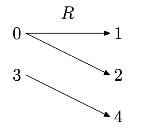
Figure \(\PageIndex{3}\) A mapping diagram for R.
It’s clear from the mapping diagram in Figure \(\PageIndex{3}\) that the number 0 in the domain is being paired (mapped) with two different range objects, namely, 1 and 2. Thus, R is not a function.
Let’s look at another example.
Is the relation described in Example \(\PageIndex{1}\) a function?
Solution
First, let’s repeat the listing of the relation T here for convenience.
\[T=\{(1,2),(3,2),(4,5)\} \nonumber \]
Next, construct a mapping diagram for the relation T. List the domain on the left, the range on the right, then use arrows to indicate the pairings, as shown in Figure \(\PageIndex{4}\).
From the mapping diagram in Figure \(\PageIndex{4}\), we can see that each domain object on the left is paired (mapped) with exactly one range object on the right. Hence, the relation T is a function.
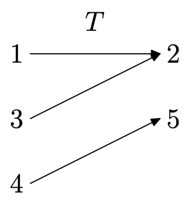
Figure \(\PageIndex{4}\). A mapping diagram for T.
Let’s look at another example.
Is the relation of Example \(\PageIndex{2}\), pictured in Figure \(\PageIndex{2}\), a function?
Solution
First, we repeat the graph of the relation from Example \(\PageIndex{2}\) here for convenience. This is shown in Figure \(\PageIndex{5}\)(a). Next, we list the ordered pairs of the relation S.
\[S=\{(1,2),(2,1),(2,4),(3,3),(4,4)\} \nonumber \]
Then we create a mapping diagram by first listing the domain on the left, the range on the right, then using arrows to indicate the pairings, as shown in Figure \(\PageIndex{5}\)(b).
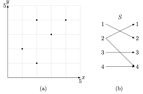
Figure \(\PageIndex{5}\) A graph of the relation S and its corresponding mapping diagram
Each object in the domain of S gets mapped to exactly one range object with one exception. The domain object 2 is paired with two range objects, namely, 1 and 4. Consequently, S is not a function.
This is a good point to summarize what we’ve learned about functions thus far.
A function consists of three parts:
- a set of objects which mathematicians call the domain,
- a second set of objects which mathematicians call the range,
- and a rule that describes how to assign a unique range object to each object in the domain.
The rule can take many forms. For example, we can use sets of ordered pairs, graphs, and mapping diagrams to describe the function. In the sections that follow, we will explore other ways of describing a function, for example, through the use of equations and simple word descriptions.
Function Notation
We’ve used the word “mapping” several times in the previous examples. This is not a word to be taken lightly; it is an important concept. In the case of the mapping diagram in Figure \(\PageIndex{5}\)(b), we would say that the number 1 in the domain of S is “mapped” (or “sent”) to the number 2 in the range of S.
There are a number of different notations we could use to indicate that the number 1 in the domain is “mapped” or “sent” to the number 2 in the range. One possible notation is
\[S : 1 \longrightarrow 2 \nonumber \]
which we would read as follows: “The relation S maps (sends) 1 to 2.” In a similar vein, we see in Figure \(\PageIndex{5}\)(b) that the domain objects 3 and 4 are mapped (sent) to the range objects 3 and 4, respectively. In symbols, we would write
\[\begin{array}{l}{S : 3 \longrightarrow 3, \text { and }} \\ {S : 4 \longrightarrow 4}\end{array} \nonumber \]
A difficulty arises when we examine what happens to the domain object 2. There are two possibilities, either
\[S : 2 \longrightarrow 1 \nonumber \] or \[S : 2 \longrightarrow 4 \nonumber \]
Which should we choose? The 1? Or the 4? Thus, S is not well-defined and is not a function, since we don’t know which range object to pair with the domain object 1.
The idea of mapping gives us an alternative way to describe a function. We could say that a function is a rule that assigns a unique object in its range to each object in its domain. Take for example, the function that maps each real number to its square. If we name the function f, then f maps 5 to 25, 6 to 36, −7 to 49, and so on. In symbols, we would write
\[f : 5 \longrightarrow 25, \quad f : 6 \longrightarrow 36, \quad \text { and } \quad f :-7 \longrightarrow 49 \nonumber \]
In general, we could write
\[f : x \longrightarrow x^{2} \nonumber \]
Note that each real number x gets mapped to a unique number in the range of f, namely, \(x^{2}\). Consequently, the function f is well defined. We’ve succeeded in writing a rule that completely defines the function f.
As another example, let’s define a function that takes a real number, doubles it, then adds 3. If we name the function g, then g would take the number 7, double it, then add 3. That is,
\[g : 7 \longrightarrow 2(7)+3 \nonumber \]
Simplifying, \(g : 7 \longrightarrow 17\). Similarly, g would take the number 9, double it, then add 3. That is,
\[g : 9 \longrightarrow 2(9)+3 \nonumber \]
Simplifying, \(g : 9 \longrightarrow 21\). In general, g takes a real number x, doubles it, then adds three. In symbols, we would write
\[g : x \longrightarrow 2 x+3 \nonumber \]
Notice that each real number x is mapped by g to a unique number in its range. Therefore, we’ve again defined a rule that completely defines the function g.
It is helpful to think of a function as a machine. The machine receives input, processes it according to some rule, then outputs a result. Something goes in (input), then something comes out (output). In the case of the function described by the rule \(f : x \longrightarrow x^{2}\), the “f-machine” receives input x, then applies its “square rule” to the input and outputs \(x^{2}\), as shown in Figure \(\PageIndex{6}\)(a). In the case of the function described by the rule \(g : x \longrightarrow 2 x+3\), the “g-machine” receives input x, then applies the rules “double,” then “add 3,” in that order, then outputs \(2x + 3\), as shown in Figure \(\PageIndex{6}\)(b).
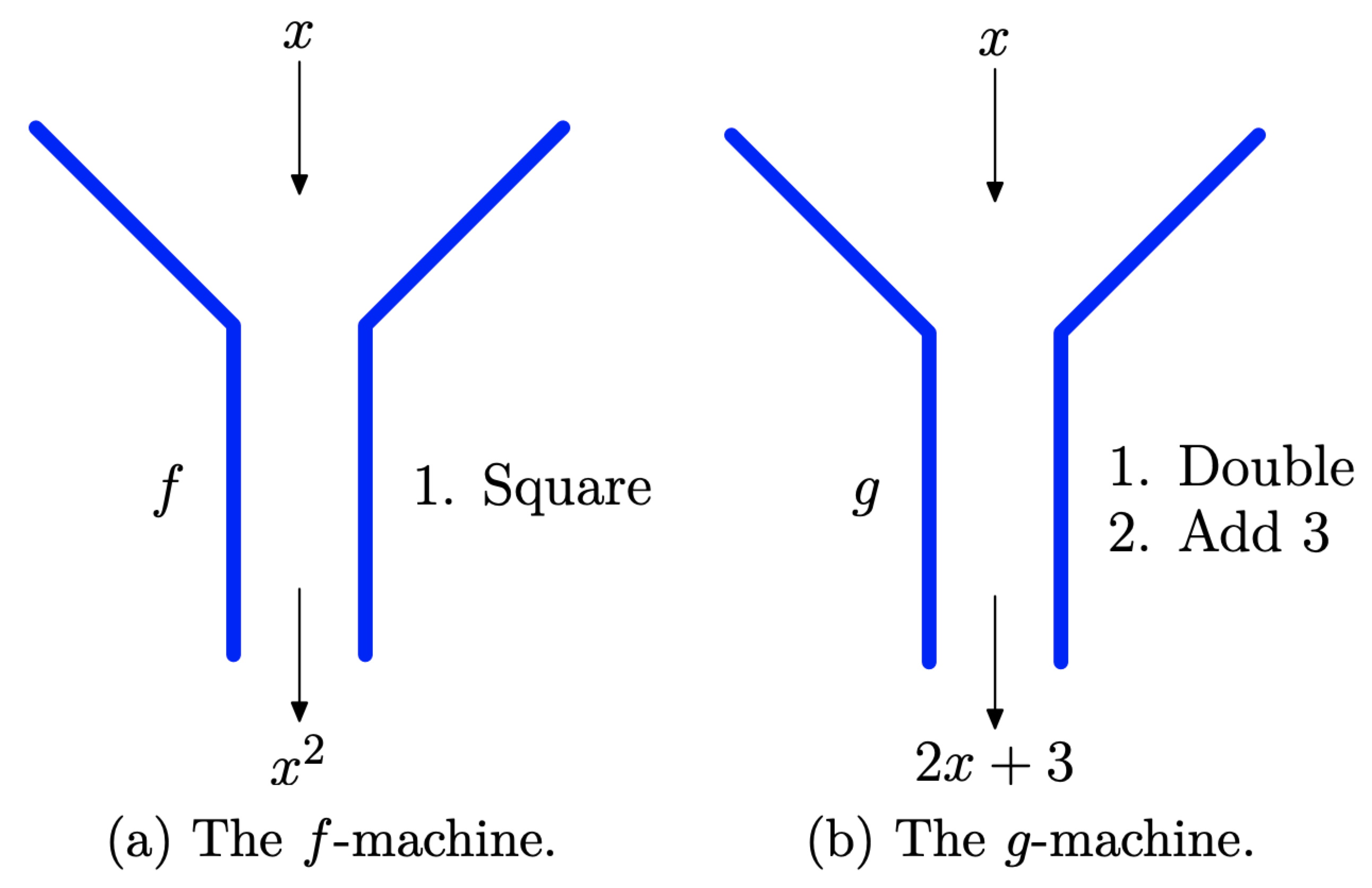
Figure \(\PageIndex{6}\) Function machines.
Let’s look at another example.
Suppose that f is defined by the following rule. For each real number x,
\[f : x \longrightarrow x^{2}-2 x-3 \nonumber \]
Where does f map the number −3? Is f a function?
Solution
We substitute −3 for x in the rule for f and obtain
\[f :-3 \longrightarrow(-3)^{2}-2(-3)-3 \nonumber \]
Simplifying,
\[f :-3 \longrightarrow 9+6-3 \nonumber \]
or,
\[f :-3 \longrightarrow 12 \nonumber \]
Thus, f maps (sends) the number −3 to the number 12. It should be clear that each real number x will be mapped (sent) to a unique real number, as defined by the rule \(f : x \longrightarrow x^{2}-2 x-3\). Therefore, f is a function.
Let’s look at another example.
Suppose that g is defined by the following rule. For each real number x that is greater than or equal to zero,
\[g : x \longrightarrow \pm \sqrt{x} \nonumber \]
Where does g map the number 4? Is g a function?
Solution
Again, we substitute 4 for x in the rule for g and obtain
\[g : 4 \longrightarrow \pm \sqrt{4} \nonumber \]
Simplifying,
\[g : 4 \longrightarrow \pm 2 \nonumber \]
Thus, g maps (sends) the number 4 to two different objects in its range, namely, 2 and −2. Consequently, g is not well-defined and is not a function.
Let’s look at another example
Suppose that we have functions f and g, defined by
\[f : x \longrightarrow x^{4}+11 \quad \text { and } \quad g : x \longrightarrow(x+2)^{2} \nonumber \]
Where does g send 5?
Solution
In this example, we see a clear advantage of function notation. Because our functions have distinct names, we can simply reference the name of the function we want our readers to use. In this case, we are asked where the function g sends the number 5, so we substitute 5 for x in
\[g : x \longrightarrow(x+2)^{2} \nonumber \]
That is,
\[g : 5 \longrightarrow(5+2)^{2} \nonumber \]
Simplifying, \(g : 5 \longrightarrow 49\).
Modern Notation
Function notation is relatively new, with some of the earliest symbolism first occurring in the 17th century. In a letter to Leibniz (1698), Johann Bernoulli wrote “For denoting any function of a variable quantity x, I rather prefer to use the capital letter having the same name X or the Greek \(\xi\), for it appears at once of what variable it is a function; this relieves the memory.”
Mathematicians are fond of the notation \[f : x \longrightarrow x^{2}-2 x \nonumber \]
because it conveys a sense of what a function does; namely, it “maps” or “sends” the number x to the number \(x^{2}-2 x\). This is what functions do, they pair each object in their domain with a unique object in their range. Equivalently, functions “send” each object in their domain to a unique object in their range.
However, in common computational situations, the “arrow” notation can be a bit clumsy, so mathematicians tend to favor a slightly different notation. Instead of writing
\[f : x \longrightarrow x^{2}-2 x \nonumber \]
mathematicians tend to favor the notation
\[f(x)=x^{2}-2 x \nonumber \]
It is important to understand from the outset that these two different notations are equivalent; they represent the same function f, one that pairs each real number x in its domain with the real number \(x^{2}-2 x\) in its range.
The first notation, \(f : x \longrightarrow x^{2}-2 x\), conveys the sense that the function f is a mapping. If we read this notation aloud, we should pronounce it as “f sends (or maps) x to \(x^{2}-2 x\).” The second notation, \(f(x) = x^{2}-2 x\), is pronounced “f of x equals \(x^{2}-2 x\).”
The phrase “f of x” is unfortunate, as our readers might recall being trained from a very early age to pair the word “of” with the operation of multiplication. For example, 1/2 of 12 is 6, as in \(1 / 2 \times 12=6\). However, in the context of function notation, even though f(x) is read aloud as “f of x,” it does not mean “f times x.” Indeed, if we remind ourselves that the notation \(f(x)=x^{2}-2 x\) is equivalent to the notation \(f : x \longrightarrow x^{2}-2 x\), then even though we might say “f of x,” we should be thinking “f sends x” or “f maps x.” We should not be thinking “f times x.”
Now, let’s see how each of these notations operates on the number 5. In the first case, using the “arrow” notation,
\[f : x \longrightarrow x^{2}-2 x \nonumber \]
To find where f sends 5, we substitute 5 for x as follows.
\[f : 5 \longrightarrow(5)^{2}-2(5) \nonumber \]
Simplifying,\(f : 5 \longrightarrow 15\). Now, because both notations are equivalent, to compute f(5), we again substitute 5 for x in
\[f(x)=x^{2}-2 x \nonumber \]
Thus,
\[f(5)=(5)^{2}-2(5) \nonumber \]
Simplifying, \(f(5)=15\). This result is read aloud as “f of 5 equals 15,” but we want to be thinking “f sends 5 to 15.”
Let’s look at examples that use this modern notation.
Given \(f(x)=x^{3}+3 x^{2}-5,\) determine \(f(-2)\)
Solution
Simply substitute −2 for x. That is,
\[\begin{aligned} f(-2) &=(-2)^{3}+3(-2)^{2}-5 \\ &=-8+3(4)-5 \\ &=-8+12-5 \\ &=-1 \end{aligned} \nonumber \]
Thus, \(f(−2) = −1\). Again, even though this is pronounced “f of −2 equals −1,” we still should be thinking “f sends −2 to −1.”
Given \[f(x)=\frac{x+3}{2 x-5} \nonumber \] determine f(6).
Solution
Simply substitute 6 for x. That is, \[\begin{aligned} f(6) &=\frac{6+3}{2(6)-5} \\ &=\frac{9}{12-5} \\ &=\frac{9}{7} \end{aligned} \nonumber \]
Thus, \(f(6) = 9/7\). Again, even though this is pronounced “f of 6 equals 9/7,” we should still be thinking “f sends 6 to 9/7.”
Given \(f(x)=5 x-3,\) determine \(f(a+2)\).
Solution
If we’re thinking in terms of mapping notation, then \[f : x \longrightarrow 5 x-3 \nonumber \]
Think of this mapping as a “machine.” Whatever we put into the machine, it first is multiplied by 5, then 3 is subtracted from the result, as shown in Figure \(\PageIndex{7}\). For example, if we put a 4 into the machine, then the function rule requires that we multiply input 4 by 5, then subtract 3 from the result. That is,
\[f : 4 \longrightarrow 5(4)-3 \nonumber \]
Simplifying, \(f : 4 \longrightarrow 17\)
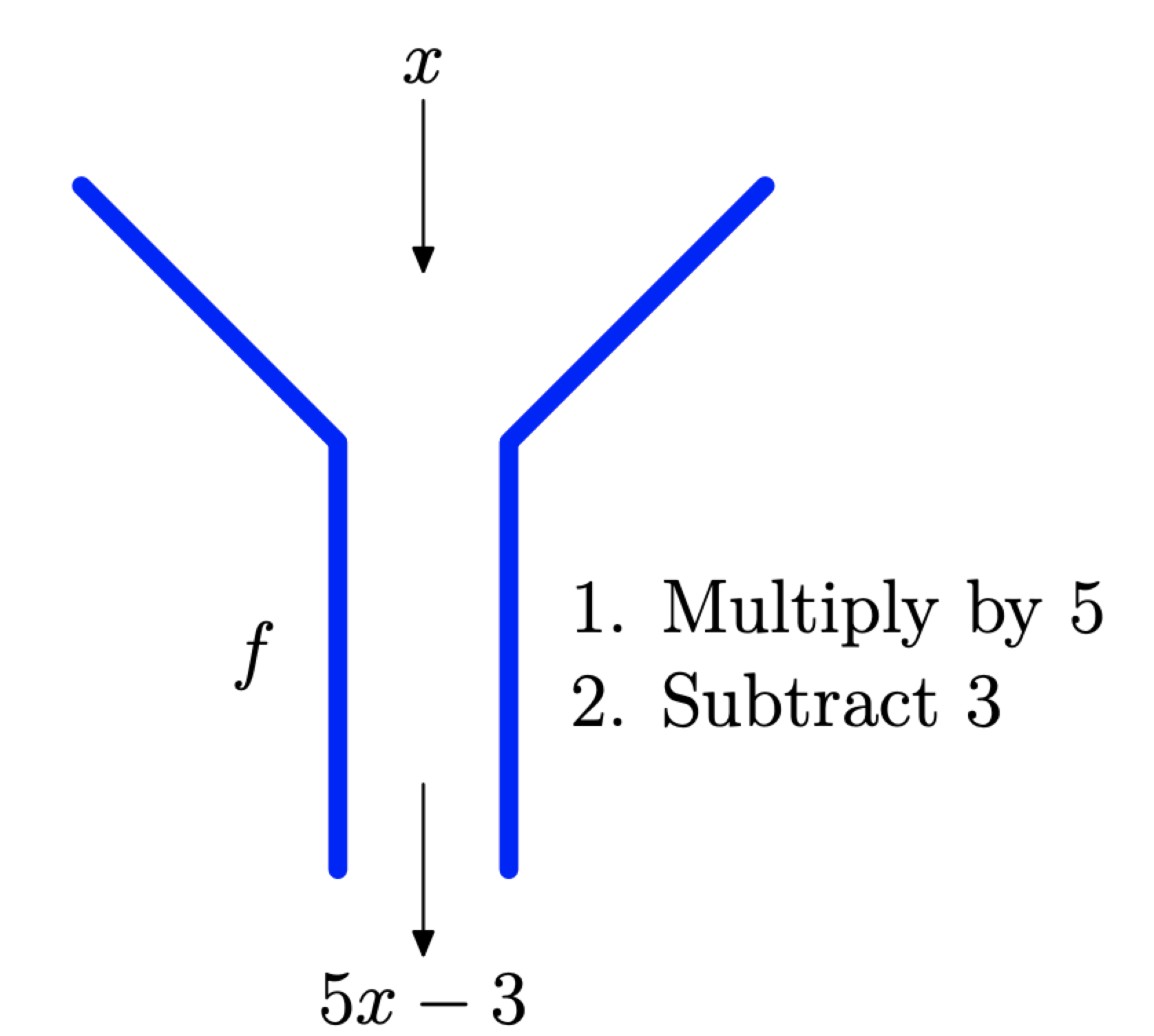
Figure \(\PageIndex{7}\). The multiply by 5 then subtract 3 machine.
Similarly, if we put an a + 2 into the machine, then the function rule requires that we multiply the input a + 2 by 5, then subtract 3 from the result. That is,
\[f : a+2 \longrightarrow 5(a+2)-3 \nonumber \]
Using modern function notation, we would write
\[f(a+2)=5(a+2)-3 \nonumber \]
Note that this is again a simple substitution, where we replace each occurrence of x in the formula \(f(x) = 5x − 3\) with the expression a + 2. Finally, use the distributive property to first multiply by 5, then subtract 3.
\[\begin{aligned} f(a+2) &=5 a+10-3 \\ &=5 a+7 \end{aligned} \nonumber \]
We will often need to substitute the result of one function evaluation into a second function for evaluation. Let’s look at an example.
Given two functions defined by \(f(x) = 3x + 2\) and \(g(x) = 5 − 4x\), find f(g(2)).
Solution
The nested parentheses in the expression f(g(2)) work in the same manner that they do with nested expressions. The rule is to work the innermost grouping symbols first, proceeding outward as you work. We’ll first evaluate g(2), then evaluate f at the result.
We begin. First, evaluate g(2) by substituting 2 for x in the defining equation \(g(x) = 5 − 4x\). Note that \(g(2) = 5 − 4(2)\), then simplify.
\[f(g(2))=f(5-4(2))=f(5-8)=f(-3) \nonumber \]
To complete the evaluation, we substitute −3 for x in the defining equation \(f(x) = 3x + 2\), then simplify.
\[f(-3)=3(-3)+2=-9+2=-7 \nonumber \]
Hence, \(f(g(2))=-7\).
It is conventional to arrange the work in one contiguous block, as follows.
\[\begin{aligned} f(g(2)) &=f(5-4(2)) \\ &=f(-3) \\ &=3(-3)+2 \\ &=-7 \end{aligned} \nonumber \]
You can shorten the task even further if you are willing to do the function substitution and simplification in your head. First, evaluate g at 2, then f at the result.
\[f(g(2))=f(-3)=-7 \nonumber \]
Let’s look at another example of this unique way of combining functions.
Given \(f(x) = 5x + 2\) and \(g(x) = 3 − 2x\), evaluate \(g(f(a))\) and simplify the result.
Solution
We work the inner function evaluation in the expression \(g(f(a))\) first. Thus, to evaluate f(a), we substitute a for x in the definition \(f(x) = 5x + 2\) to get
\[g(f(a))=g(5 a+2) \nonumber \]
Now we need to evaluate \(g(5a + 2)\). To do this, we substitute \(5a + 2\) for x in the definition \(g(x) = 3 − 2x\) to get
\[g(5 a+2)=3-2(5 a+2) \nonumber \]
We can expand this last result and simplify. Thus,
\[g(f(a))=3-10 a-4=-10 a-1 \nonumber \]
Again, it is conventional to arrange the work in one continuous block, as follows.
\[\begin{aligned} g(f(a)) &=g(5 a+2) \\ &=3-2(5 a+2) \\ &=3-10 a-4 \\ &=-10 a-1 \end{aligned} \nonumber \]
Hence, \(g(f(a))=-10 a-1\).
Extracting the Domain of a Function
We’ve seen that the domain of a relation or function is the set of all the first coordinates of its ordered pairs. However, if a functional relationship is defined by an equation such as \(f(x) = 3x − 4\), then it is not practical to list all ordered pairs defined by this relationship. For any real x-value, you get an ordered pair. For example, if x = 5, then \(f(5) = 3(5) − 4 = 11\), leading to the ordered pair (5, f(5)) or (5, 11). As you can see, the number of such ordered pairs is infinite. For each new x-value, we get another function value and another ordered pair.
Therefore, it is easier to turn our attention to the values of x that yield real number responses in the equation \(f(x) = 3x − 4\). This leads to the following key idea.
If a function is defined by an equation, then the domain of the function is the set of “permissible x-values,” the values that produce a real number response defined by the equation.
We sometimes like to say that the domain of a function is the set of “OK x-values to use in the equation.” For example, if we define a function with the rule \(f(x) = 3x − 4\), it is immediately apparent that we can use any value we want for x in the rule \(f(x) = 3x − 4\). Thus, the domain of f is all real numbers. We can write that the domain \(D=\mathbb{R}\), or we can use interval notation and write that the domain \(D=(-\infty, \infty)\).
It is not the case that x can be any real number in the function defined by the rule \(f(x)=\sqrt{x}\). It is not possible to take the square root of a negative number.2 Therefore, x must either be zero or a positive real number. In set-builder notation, we can describe the domain with \(D=\{x : x \geq 0\}\). In interval notation, we write \(D=[0, \infty)\).
We must also be aware of the fact that we cannot divide by zero. If we define a function with the rule \(f(x)=x /(x-3)\), we immediately see that x = 3 will put a zero in the denominator. Division by zero is not defined. Therefore, 3 is not in the domain of f. No other x-value will cause a problem. The domain of f is best described with set-builder notation as \(D=\{x : x \neq 3\}\).
Functions Without Formulae
In the previous section, we defined functions by means of a formula, for example, as in
\[f(x)=\frac{x+3}{2-3 x} \nonumber \]
Euler would be pleased with this definition, for as we have said previously, Euler thought of functions as analytic expressions.
However, it really isn’t necessary to provide an expression or formula to define a function. There are other forms we can use to express a functional relationship: a graph, a table, or even a narrative description. The only thing that is really important is the requirement that the function be well-defined, and by “well-defined,” we mean that each object in the function’s domain is paired with one and only one object in its range.
As an example, let’s look at a special function \(\pi\) on the natural numbers,3 which returns the number of primes less than or equal to a given natural number. For example, the primes less than or equal to the number 23 are 2, 3, 5, 7, 11, 13, 17, 19, and 23, nine numbers in all. Therefore, the number of primes less than or equal to 23 is nine. In symbols, we would write
\[\pi(23)=9 \nonumber \]
Note the absence of a formula in the definition of this function. Indeed, the definition is descriptive in nature, so we might write
\[\pi(n)=\text { number of primes less than or equal to } n \nonumber \]
The important thing is not how we define this special function \(π\), but the fact that it is well-defined; that is, for each natural number \(n\), there are a fixed number of primes less than or equal to \(n\). Thus, each natural number in the domain of \(π\) is paired with one and only one number in its range.
Now, just because our function doesn’t provide an expression for calculating the number of primes less than or equal to a given natural number n, it doesn’t stop mathematicians from seeking such a formula. Euclid of Alexandria (325-265 BC), a Greek mathematician, proved that the number of primes is infinite, but it was the German mathematician and scientist, Johann Carl Friedrich Gauss (1777-1855), who first proposed that the number of primes less than or equal to n can be approximated by the formula
\[\pi(n) \approx \frac{n}{\ln n} \nonumber \]
where ln n is the “natural logarithm” of n (to be explained in Chapter 9). This approximation gets better and better with larger and larger values of n. The formula was refined by Gauss, who did not provide a proof, and the problem became known as the Prime Number Theorem. It was not until 1896 that Jacques Salomon Hadamard (1865-1963) and Charles Jean Gustave Nicolas Baron de la Vallee Poussin (1866-1962), working independently, provided a proof of the Prime Number Theorem.