3.3: Equations of Lines
- Page ID
- 19694
\( \newcommand{\vecs}[1]{\overset { \scriptstyle \rightharpoonup} {\mathbf{#1}} } \)
\( \newcommand{\vecd}[1]{\overset{-\!-\!\rightharpoonup}{\vphantom{a}\smash {#1}}} \)
\( \newcommand{\dsum}{\displaystyle\sum\limits} \)
\( \newcommand{\dint}{\displaystyle\int\limits} \)
\( \newcommand{\dlim}{\displaystyle\lim\limits} \)
\( \newcommand{\id}{\mathrm{id}}\) \( \newcommand{\Span}{\mathrm{span}}\)
( \newcommand{\kernel}{\mathrm{null}\,}\) \( \newcommand{\range}{\mathrm{range}\,}\)
\( \newcommand{\RealPart}{\mathrm{Re}}\) \( \newcommand{\ImaginaryPart}{\mathrm{Im}}\)
\( \newcommand{\Argument}{\mathrm{Arg}}\) \( \newcommand{\norm}[1]{\| #1 \|}\)
\( \newcommand{\inner}[2]{\langle #1, #2 \rangle}\)
\( \newcommand{\Span}{\mathrm{span}}\)
\( \newcommand{\id}{\mathrm{id}}\)
\( \newcommand{\Span}{\mathrm{span}}\)
\( \newcommand{\kernel}{\mathrm{null}\,}\)
\( \newcommand{\range}{\mathrm{range}\,}\)
\( \newcommand{\RealPart}{\mathrm{Re}}\)
\( \newcommand{\ImaginaryPart}{\mathrm{Im}}\)
\( \newcommand{\Argument}{\mathrm{Arg}}\)
\( \newcommand{\norm}[1]{\| #1 \|}\)
\( \newcommand{\inner}[2]{\langle #1, #2 \rangle}\)
\( \newcommand{\Span}{\mathrm{span}}\) \( \newcommand{\AA}{\unicode[.8,0]{x212B}}\)
\( \newcommand{\vectorA}[1]{\vec{#1}} % arrow\)
\( \newcommand{\vectorAt}[1]{\vec{\text{#1}}} % arrow\)
\( \newcommand{\vectorB}[1]{\overset { \scriptstyle \rightharpoonup} {\mathbf{#1}} } \)
\( \newcommand{\vectorC}[1]{\textbf{#1}} \)
\( \newcommand{\vectorD}[1]{\overrightarrow{#1}} \)
\( \newcommand{\vectorDt}[1]{\overrightarrow{\text{#1}}} \)
\( \newcommand{\vectE}[1]{\overset{-\!-\!\rightharpoonup}{\vphantom{a}\smash{\mathbf {#1}}}} \)
\( \newcommand{\vecs}[1]{\overset { \scriptstyle \rightharpoonup} {\mathbf{#1}} } \)
\(\newcommand{\longvect}{\overrightarrow}\)
\( \newcommand{\vecd}[1]{\overset{-\!-\!\rightharpoonup}{\vphantom{a}\smash {#1}}} \)
\(\newcommand{\avec}{\mathbf a}\) \(\newcommand{\bvec}{\mathbf b}\) \(\newcommand{\cvec}{\mathbf c}\) \(\newcommand{\dvec}{\mathbf d}\) \(\newcommand{\dtil}{\widetilde{\mathbf d}}\) \(\newcommand{\evec}{\mathbf e}\) \(\newcommand{\fvec}{\mathbf f}\) \(\newcommand{\nvec}{\mathbf n}\) \(\newcommand{\pvec}{\mathbf p}\) \(\newcommand{\qvec}{\mathbf q}\) \(\newcommand{\svec}{\mathbf s}\) \(\newcommand{\tvec}{\mathbf t}\) \(\newcommand{\uvec}{\mathbf u}\) \(\newcommand{\vvec}{\mathbf v}\) \(\newcommand{\wvec}{\mathbf w}\) \(\newcommand{\xvec}{\mathbf x}\) \(\newcommand{\yvec}{\mathbf y}\) \(\newcommand{\zvec}{\mathbf z}\) \(\newcommand{\rvec}{\mathbf r}\) \(\newcommand{\mvec}{\mathbf m}\) \(\newcommand{\zerovec}{\mathbf 0}\) \(\newcommand{\onevec}{\mathbf 1}\) \(\newcommand{\real}{\mathbb R}\) \(\newcommand{\twovec}[2]{\left[\begin{array}{r}#1 \\ #2 \end{array}\right]}\) \(\newcommand{\ctwovec}[2]{\left[\begin{array}{c}#1 \\ #2 \end{array}\right]}\) \(\newcommand{\threevec}[3]{\left[\begin{array}{r}#1 \\ #2 \\ #3 \end{array}\right]}\) \(\newcommand{\cthreevec}[3]{\left[\begin{array}{c}#1 \\ #2 \\ #3 \end{array}\right]}\) \(\newcommand{\fourvec}[4]{\left[\begin{array}{r}#1 \\ #2 \\ #3 \\ #4 \end{array}\right]}\) \(\newcommand{\cfourvec}[4]{\left[\begin{array}{c}#1 \\ #2 \\ #3 \\ #4 \end{array}\right]}\) \(\newcommand{\fivevec}[5]{\left[\begin{array}{r}#1 \\ #2 \\ #3 \\ #4 \\ #5 \\ \end{array}\right]}\) \(\newcommand{\cfivevec}[5]{\left[\begin{array}{c}#1 \\ #2 \\ #3 \\ #4 \\ #5 \\ \end{array}\right]}\) \(\newcommand{\mattwo}[4]{\left[\begin{array}{rr}#1 \amp #2 \\ #3 \amp #4 \\ \end{array}\right]}\) \(\newcommand{\laspan}[1]{\text{Span}\{#1\}}\) \(\newcommand{\bcal}{\cal B}\) \(\newcommand{\ccal}{\cal C}\) \(\newcommand{\scal}{\cal S}\) \(\newcommand{\wcal}{\cal W}\) \(\newcommand{\ecal}{\cal E}\) \(\newcommand{\coords}[2]{\left\{#1\right\}_{#2}}\) \(\newcommand{\gray}[1]{\color{gray}{#1}}\) \(\newcommand{\lgray}[1]{\color{lightgray}{#1}}\) \(\newcommand{\rank}{\operatorname{rank}}\) \(\newcommand{\row}{\text{Row}}\) \(\newcommand{\col}{\text{Col}}\) \(\renewcommand{\row}{\text{Row}}\) \(\newcommand{\nul}{\text{Nul}}\) \(\newcommand{\var}{\text{Var}}\) \(\newcommand{\corr}{\text{corr}}\) \(\newcommand{\len}[1]{\left|#1\right|}\) \(\newcommand{\bbar}{\overline{\bvec}}\) \(\newcommand{\bhat}{\widehat{\bvec}}\) \(\newcommand{\bperp}{\bvec^\perp}\) \(\newcommand{\xhat}{\widehat{\xvec}}\) \(\newcommand{\vhat}{\widehat{\vvec}}\) \(\newcommand{\uhat}{\widehat{\uvec}}\) \(\newcommand{\what}{\widehat{\wvec}}\) \(\newcommand{\Sighat}{\widehat{\Sigma}}\) \(\newcommand{\lt}{<}\) \(\newcommand{\gt}{>}\) \(\newcommand{\amp}{&}\) \(\definecolor{fillinmathshade}{gray}{0.9}\)In this section we will develop the slope-intercept form of a line. When you have completed the work in this section, you should be able to look at the graph of a line and determine its equation in slope-intercept form.
The Slope-Intercept Form
In the previous section, we developed the formula for the slope of a line. Let’s assume that the dependent variable is y and the independent variable is x and we have a line passing through the points \(P\left(x_{1}, y_{1}\right)\) and \(Q\left(x_{2}, y_{2}\right)\), as shown in Figure \(\PageIndex{1}\).
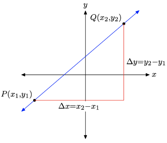
As we sweep our eyes from left to right, note that the change in x is \(\Delta x=x_{2}-x_{1}\) and the change in y is \(\Delta y=y_{2}-y_{1}\). Thus, the slope of the line is determined by the formula
\[\text { Slope }=\frac{\Delta y}{\Delta x}=\frac{y_{2}-y_{1}}{x_{2}-x_{1}} \nonumber \]
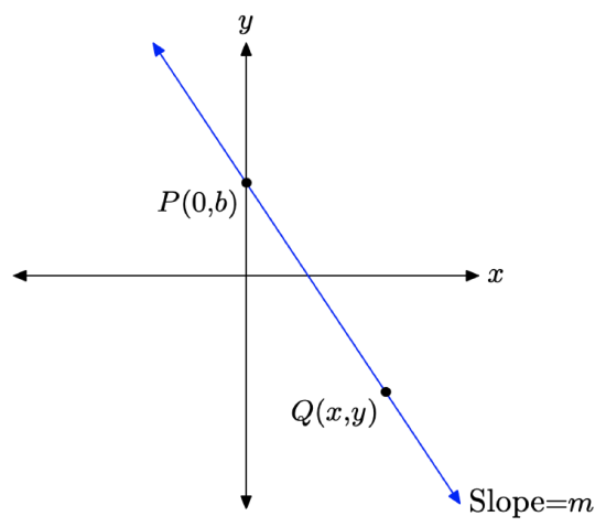
Now consider the line in Figure \(\PageIndex{2}\). Suppose that we are given two facts about this line:
- The point where the line crosses the y-axis (the y-intercept) is (0, b).
- The “slope” of the line is some number m.
To find the equation of the line pictured in Figure \(\PageIndex{2}\), select an arbitrary point Q(x, y) on the line, then compute the slope of the line using \(\left(x_{1}, y_{1}\right)=P(0, b)\) and \(\left(x_{2}, y_{2}\right)=Q(x, y)\) in the slope formula (1).
\[\text { Slope }=\frac{y_{2}-y_{1}}{x_{2}-x_{1}}=\frac{y-b}{x-0} \nonumber \]
Simplify.
\[\text { Slope }=\frac{y-b}{x} \nonumber \]
We’re given that the slope is the number m, so substitute this number for the word “Slope” in the last result.
\[m=\frac{y-b}{x} \nonumber \]
Multiply both sides of the last equation by \(x\).
\[m x=y-b \nonumber \]
Add b to both sides of the last equation to obtain
\[m x+b=y \nonumber \]
or upon exchanging sides of the equation,
\[y=m x+b \nonumber \]
The above discussion leads to the following result.
If the line \(L\) intercepts the y-axis at the point (0, b) and has slope m, then the equation of the line is
\[y=m x+b. \label{slopeintercept eq} \]
This form of the equation of a line is called the slope-intercept form. The function defined by the equation \[f(x)=m x+b \nonumber \] is called a linear function.
It is important to note two key facts about the slope-intercept form y = mx + b.
- The coefficient of x (the m in y = mx + b) is the slope of the line.
- The constant term (the b in y = mx+b) is the y-coordinate of the y-intercept (0, b).
When given the slope of a line and the y-intercept of the line, use the slope-intercept form as follows:
- Substitute the given slope for m in the formula \(y = mx + b\).
- Substitute the y-coordinate of the y-intercept for b in the formula \(y = mx + b\).
For example, if the line has slope −2 and the y-intercept (the point where the line crosses the y-axis) is (0, 3), then substitute m = −2 and b = 3 into Equation \ref{slopeintercept eq} to obtain
\[y = −2x + 3 \nonumber \].
Let’s look at some examples of use of this all-important formula.
What is the equation of the line having slope −2/3 and y-intercept at (0, 3)? Sketch the line on graph paper.
Solution
The equation of the line is
\[y=m x+b \nonumber \]
We’re given that the slope is −2/3. Hence, m = −2/3. Secondly, we’re given that the line intercepts the y-axis at the point (0, 3). In the slope-intercept form y = mx + b, recall that b represents the y-coordinate of the y-intercept. Hence, b = 3. Substitute m = −2/3 and b = 3 in equation (4), obtaining
\[y=-\frac{2}{3} x+3 \nonumber \]
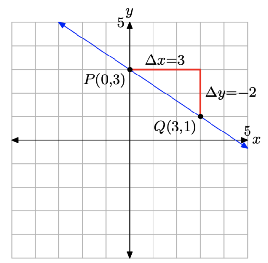
To sketch the graph of the line, first locate the y-intercept at P(0, 3), as shown in Figure \(\PageIndex{3}\). Starting from the y-intercept at P(0, 3), move 3 units to the right and 2 units downward to the point Q(3, 1). The required line passes through the points P and Q.
Note that the line “intercepts” the y-axis at 3 and slants downhill, in accordance with the fact that the slope is negative in this example.
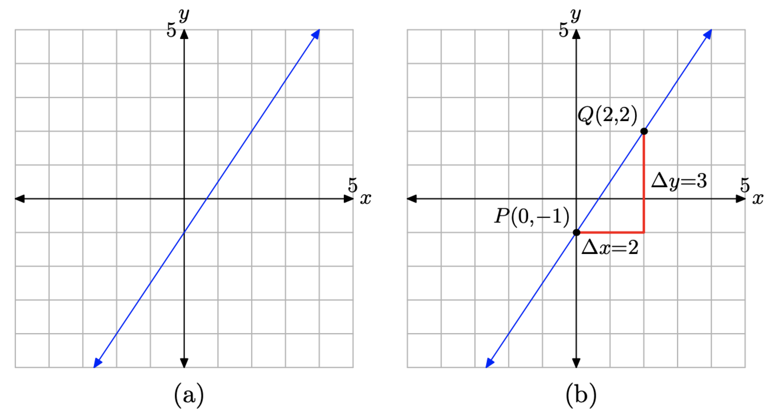
Given the graph of the line in Figure \(\PageIndex{4}\)(a), determine the equation of the line.
Solution
First, locate the y-intercept of the line, which we’ve labeled P(0, −1) in Figure \(\PageIndex{4}\)(b). In the formula y = mx + b, recall that b represents the y-coordinate of the y-intercept. Thus, b = −1.
Secondly, we need to determine the slope of the line. In Figure \(\PageIndex{4}\)(b), start at the point P, move 2 units to the right, then 3 units upward to the point Q(2, 2). This makes the slope \[m=\frac{\Delta y}{\Delta x}=\frac{3}{2} \nonumber \]
Substitute m = 3/2 and b = −1 into the slope-intercept form y = mx + b to obtain
\[y=\frac{3}{2} x-1 \nonumber \]
which is the desired equation of the line.
Making Connections
If the connection between rate and slope is still not clear, let’s recall an example we did earlier in the chapter.
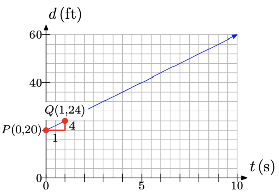
Sebastian waves good-bye to his brother, who is talking to a group of his friends approximately 20 feet away. Sebastian then begins to walk away from his brother at a constant rate of 4 feet per second.
The distance between the brothers depends upon the amount of time that has passed, so we set distance d on the vertical axis and time t on the horizontal axis, as shown in Figure \(\PageIndex{5}\). Note that d and t are taking the “usual” place of y and x, respectively. The distance separating the brothers at time t = 0 is d = 20 feet. This is indicated with the “d-intercept” at P(0, 20) in Figure \(\PageIndex{5}\).
Next, the distance between the brothers is increasing at a rate of 4 feet per second. Starting at the point P(0, 20), move 1 second to the right (2 boxes) and 4 units up (1 box) to the point Q(1, 24), as shown in Figure \(\PageIndex{5}\). The line through the points P and Q then models the distance between the brothers as a function of time.
If you recall, we then determined a relation between distance d and time t by examining the distance between the brothers at times t = 0, 1, 2, and 3, and summarizing the results in Table \(\PageIndex{1}\).
| t | d |
|---|---|
| 0 | 20 |
| 1 | 20+4(1) |
| 2 | 20+4(2) |
| 3 | 20+4(3) |
Intuition then led to the following model, which provides the distance d between the brothers as a function of time t.
\[d=20+4 t \nonumber \]
Again, readers should check that equation (6) produces the results in Table \(\PageIndex{1}\) at t = 0, 1, 2, and 3.
Alternatively, with the theory developed in this section, we would develop the equation of the line by using the slope-intercept form of the line; that is,
\[y=m x+b \nonumber \]
However, in this case, the dependent variable is d, not y, and the independent variable is t, not x. So, replace y and x in equation (7) with d and t, respectively, obtaining
\[d=m t+b \nonumber \]
Next, the line intercepts the d-axis at P(0, 20), so b = 20. Furthermore, the slope of the line is 4 feet per second, so m = 4. Substitute m = 4 and b = 20 in equation (8) to obtain
\[d=4 t+20 \nonumber \]
or using function notation, \(d(t) = 4t + 20\). Note that equation (9) is identical to the intuitively generated model of equation (6).
Hopefully, this development should cement for all time the idea that slope of the line is the rate at which the dependent variable is changing with respect to the independent variable.
The Standard Form of a Line
We now know that if our equation has the form \(y=m x+b\) (or can be manipulated into this form), the graph will be a line. Let’s take a moment to demonstrate that the graph of the equation \(A x+B y=C\), where A, B, and C are constants, is a line.
If we can place the form \(A x+B y=C\) into slope-intercept form \(y=m x+b\), then that will demonstrate that the graph of \(A x+B y=C\) is a line. So, start with \(A x+B y=C\) and subtract Ax from both sides of the equation.
\[B y=-A x+C \nonumber \]
Divide both sides of this last equation by B. Note that there is an assumption here that \(B \neq 0\). We will handle the case when B = 0 separately, at the end of this section.
\[\begin{aligned} \frac{B y}{B} &=\frac{-A x+C}{B} \\ y &=-\frac{A}{B} x+\frac{C}{B} \end{aligned} \nonumber \]
When we compare \(y=-(A / B) x+(C / B)\) with y = mx + b, we note that the slope is m = −A/B and the y-coordinate of the y-intercept is b = C/B. Because we were successful in placing the equation \(A x+B y=C\) into slope-intercept form, we now know that the graph of \(A x+B y=C\) is a line (we’ll need this result in later work).
The graph of the equation Ax + By = C is a line. The form \[A x+B y=C \nonumber \] is called the standard form of a line.
Let’s look at an example.
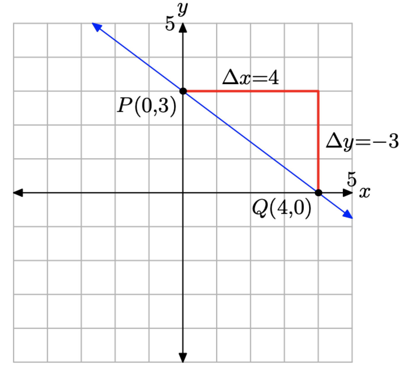
The equation 3x+4y = 12 is in standard form. Place this equation in slope-intercept form, determine the slope and y-intercept, then use these results to draw the graph of the line.
Solution
First, solve the equation 3x + 4y = 12 for y.
\[\begin{aligned} 3 x+4 y &=12 \\ 4 y &=-3 x+12 \\ y &=-\frac{3}{4} x+3 \end{aligned} \nonumber \]
Note in the last step how the distributive property came into play. When we divided −3x + 12 by 4, we divided each term by 4, getting (−3/4)x + 3.
When we compare y = (−3/4)x+3 with the general slope-intercept form y = mx+b, we determine that the slope is m = −3/4 and the y-coordinate of the y-intercept is b = 3. To sketch the graph of the line, as we’ve done in Figure \(\PageIndex{6}\), plot the y-intercept at P(0, 3), then move 4 units to the right and 3 units down to the point Q(4, 0). The line passing through the points P and Q is the required line.
Note again that the slope is m = −3/4 and the line slants “downhill.” Also, b = 3 and the line “intercepts” the y-axis at P(0, 3).
Let’s look at another example.
In Example \(\PageIndex{1}\), we determined that the given line had the equation
\[y=\frac{3}{2} x-1 \nonumber \]
Place this equation in standard from \(Ax + By = C\), where A, B, and C are integers and \(A > 0\).
Solution
We’re requested to place the equation \(y = (3/2)x − 1\) in the form \(Ax + By = C\), where A, B, and C are integers, so let’s begin by clearing fractions from the equation. Multiply both sides of the equation by the common denominator 2.
\[\begin{aligned} y &=\frac{3}{2} x-1 \\ 2 y &=2\left(\frac{3}{2} x-1\right) \\ 2 y &=3 x-2 \end{aligned} \nonumber \]
Now, subtract 2y from both sides of the equation, then add 2 to both sides of the equation to obtain
\[2=3 x-2 y \nonumber \]
or equivalently,
\[3 x-2 y=2 \nonumber \]
Note that this last result is in standard form \(Ax + By = C\), where A, B, and C are integers and A > 0.
Intercepts
We now know that the graph of the equation \(Ax + By = C\), where A, B, and C are constants, is a line. Because the graph of \(Ax + By = C\) is a line, to draw the graph of the line, we need only find two points that satisfy the equation, plot them, then draw a line through them. Our two favorite points to work with are the x- and y-intercepts, because each involves the number zero, an easy number to work with.
Consider the graph in Figure \(\PageIndex{7}\)(a). Note that the graph passes through the x-axis three times. The points where the graph intercepts the x-axis are called x-intercepts. Note that each of these points has a defining value in common: the y-value of each of these x-intercepts is equal to zero.
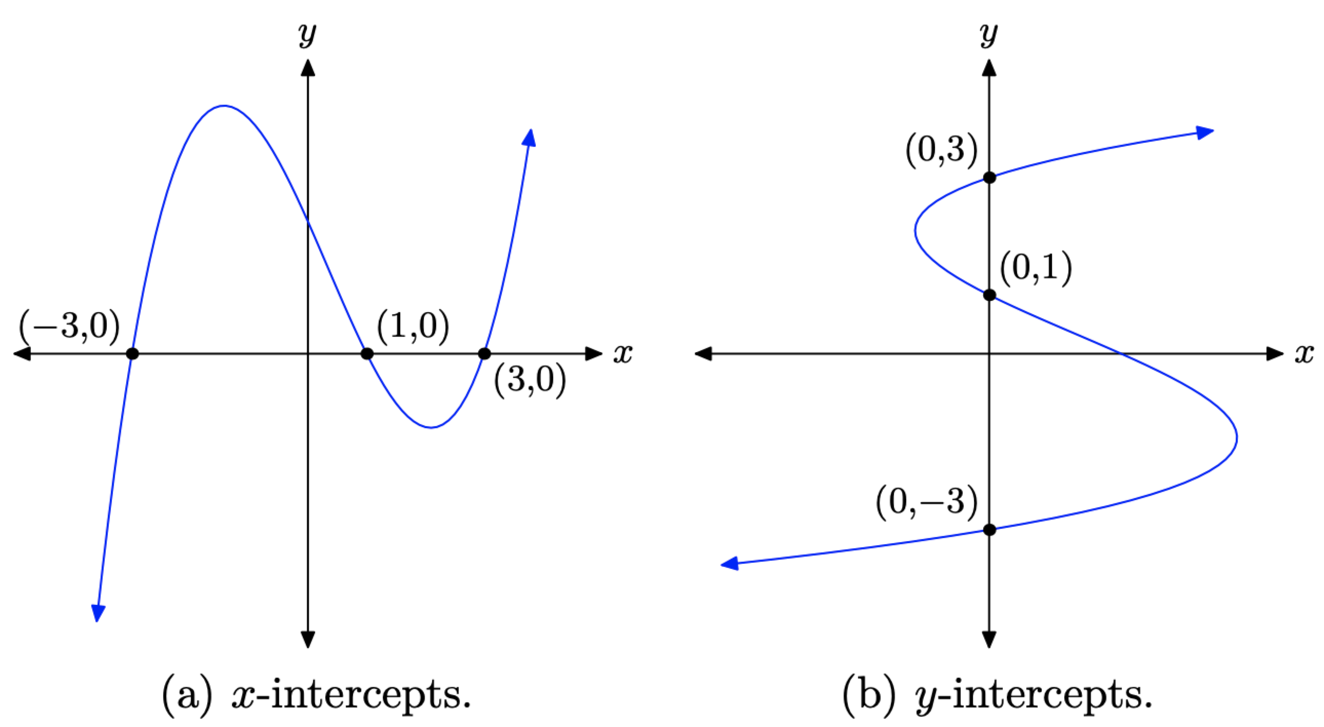
To find an x intercept, let y = 0 in the equation and solve for x.
On the other hand, consider the graph in Figure \(\PageIndex{7}\)(b). Note that this is not a function (fails the vertical line test) but the graph intercepts the y-axis three separate times. The points where the graph intercepts the y-axis are called y-intercepts. Note that each of the y-intercepts in Figure \(\PageIndex{7}\)(b) has a defining value in common: the x-value of each of the y-intercepts is equal to zero.
To find a y-intercept, let x = 0 in the equation and solve for y.
Let’s put what we’ve learned into practice.
Sketch the graph of 3x + 4y = 12.
Solution
We drew the graph of the equation 3x + 4y = 12 in Figure \(\PageIndex{6}\). There we solved the equation for y to determine the slope and the y-intercept. These, in turn, were used to draw the graph of 3x + 4y = 12 in Figure \(\PageIndex{6}\).
Here, our approach will be different. We will first determine the x- and y-intercepts, plot them, then draw a line through these intercepts. Hopefully, we will get a result that matches that in Figure \(\PageIndex{6}\).
To find the x-intercept, let \(y = 0\) in \(3x + 4y = 12\) and solve for x.
\[\begin{aligned} 3 x+4 y &=12 \\ 3 x+4(0) &=12 \\ 3 x &=12 \\ x &=4 \end{aligned} \nonumber \]
Hence, the x-intercept is the point Q(4, 0). To find the y-intercept, let x = 0 in \(3x + 4y = 12\) and solve for y.
\[\begin{aligned} 3 x+4 y &=12 \\ 3(0)+4 y &=12 \\ 4 y &=12 \\ y &=3 \end{aligned} \nonumber \]
Hence, the y-intercept is the point P(0, 3). In Figure \(\PageIndex{8}\), we’ve plotted both x- and y-intercepts and drawn a line through them. Note that the resulting line in Figure \(\PageIndex{8}\) matches the same line drawn in Figure \(\PageIndex{6}\) (where we used a different method).
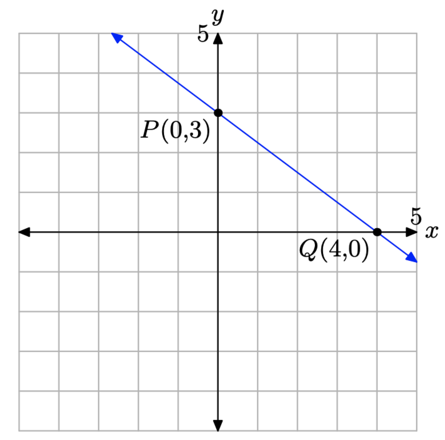
Figure \(\PageIndex{8}\). Plotting the x- and y-intercepts.
We recommend that whenever the line is given in Standard Form \(Ax + By = C\), find the x- and y-intercepts, plot them, then draw a line through them. This technique is quite efficient because working with the number zero greatly simplifies the calculations.
Horizontal and Vertical Lines
We’ve introduced the standard form of the line \(Ax + By = C\). The case where A and B are simultaneously equal to zero is not very interesting.4 However, the following two cases are of interest.
- If we let A = 0 and B 6= 0 in the standard form \(Ax + By = C\), then By = C, or equivalently y = C/B. Note that this has the form y = b, where b is some constant.
- Similarly, if we let B = 0 and A 6= 0 in the standard form \(Ax + By = C\), then Ax = C, or equivalently, x = C/A. Note that this has the form x = a, where a is some constant.
The lines having the form x = a and y = b are two of the easiest lines to plot. Let’s look at an example of each.
Sketch the graph of the equation x = 3.
Solution
The direction “sketch the graph of the equation x = 3” can be quite vexing unless one remembers that a graph of an equation is the set of all points that satisfy the equation. Thus, the direction is better posed if we say “sketch the set of all points (x, y) that satisfy x = 3,” or equivalently, “sketch the set of all points (x, y) that have an x-value of 3.” Then it is an easy matter to sketch the vertical line shown in Figure \(\PageIndex{9}\).
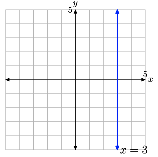
Note that each point on the line has an x-value equal to 3. Also, note that the slope of this vertical line is undefined.
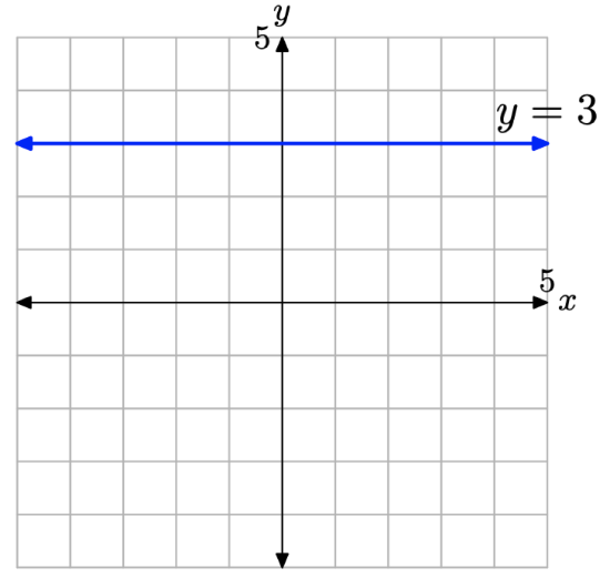
Sketch the graph of the equation y = 3.
Solution
This direction is better posed if we say “sketch the set of all points (x, y) that satisfy y = 3,” or equivalently, “sketch the set of all points (x, y) that have a y-value of 3.” Then it is an easy matter to sketch the horizontal line shown in Figure \(\PageIndex{10}\).
Note that each point on the line has a y-value equal to 3. Also, note that this horizontal line has slope zero.
Two final comments are in order. Because the line in Figure 10 has slope zero and y-intercept (0, 3), we can insert m = 0 and b = 3 into the slope intercept form y = mx + b and obtain
\[y=0 x+3 \nonumber \]
which of course, is equivalent to y = 3. However, the vertical line shown in Figure \(\PageIndex{9}\) has “undefined” slope, so this approach is unavailable. We must simply recognize that the vertical line in Figure \(\PageIndex{9}\) consists of all points having an x-value equal to 3, and then intuit that its equation is x = 3.


