
8.1: Exponents and Roots
- Page ID
- 19727

\( \newcommand{\vecs}[1]{\overset { \scriptstyle \rightharpoonup} {\mathbf{#1}} } \)
\( \newcommand{\vecd}[1]{\overset{-\!-\!\rightharpoonup}{\vphantom{a}\smash {#1}}} \)
\( \newcommand{\dsum}{\displaystyle\sum\limits} \)
\( \newcommand{\dint}{\displaystyle\int\limits} \)
\( \newcommand{\dlim}{\displaystyle\lim\limits} \)
\( \newcommand{\id}{\mathrm{id}}\) \( \newcommand{\Span}{\mathrm{span}}\)
( \newcommand{\kernel}{\mathrm{null}\,}\) \( \newcommand{\range}{\mathrm{range}\,}\)
\( \newcommand{\RealPart}{\mathrm{Re}}\) \( \newcommand{\ImaginaryPart}{\mathrm{Im}}\)
\( \newcommand{\Argument}{\mathrm{Arg}}\) \( \newcommand{\norm}[1]{\| #1 \|}\)
\( \newcommand{\inner}[2]{\langle #1, #2 \rangle}\)
\( \newcommand{\Span}{\mathrm{span}}\)
\( \newcommand{\id}{\mathrm{id}}\)
\( \newcommand{\Span}{\mathrm{span}}\)
\( \newcommand{\kernel}{\mathrm{null}\,}\)
\( \newcommand{\range}{\mathrm{range}\,}\)
\( \newcommand{\RealPart}{\mathrm{Re}}\)
\( \newcommand{\ImaginaryPart}{\mathrm{Im}}\)
\( \newcommand{\Argument}{\mathrm{Arg}}\)
\( \newcommand{\norm}[1]{\| #1 \|}\)
\( \newcommand{\inner}[2]{\langle #1, #2 \rangle}\)
\( \newcommand{\Span}{\mathrm{span}}\) \( \newcommand{\AA}{\unicode[.8,0]{x212B}}\)
\( \newcommand{\vectorA}[1]{\vec{#1}} % arrow\)
\( \newcommand{\vectorAt}[1]{\vec{\text{#1}}} % arrow\)
\( \newcommand{\vectorB}[1]{\overset { \scriptstyle \rightharpoonup} {\mathbf{#1}} } \)
\( \newcommand{\vectorC}[1]{\textbf{#1}} \)
\( \newcommand{\vectorD}[1]{\overrightarrow{#1}} \)
\( \newcommand{\vectorDt}[1]{\overrightarrow{\text{#1}}} \)
\( \newcommand{\vectE}[1]{\overset{-\!-\!\rightharpoonup}{\vphantom{a}\smash{\mathbf {#1}}}} \)
\( \newcommand{\vecs}[1]{\overset { \scriptstyle \rightharpoonup} {\mathbf{#1}} } \)
\(\newcommand{\longvect}{\overrightarrow}\)
\( \newcommand{\vecd}[1]{\overset{-\!-\!\rightharpoonup}{\vphantom{a}\smash {#1}}} \)
\(\newcommand{\avec}{\mathbf a}\) \(\newcommand{\bvec}{\mathbf b}\) \(\newcommand{\cvec}{\mathbf c}\) \(\newcommand{\dvec}{\mathbf d}\) \(\newcommand{\dtil}{\widetilde{\mathbf d}}\) \(\newcommand{\evec}{\mathbf e}\) \(\newcommand{\fvec}{\mathbf f}\) \(\newcommand{\nvec}{\mathbf n}\) \(\newcommand{\pvec}{\mathbf p}\) \(\newcommand{\qvec}{\mathbf q}\) \(\newcommand{\svec}{\mathbf s}\) \(\newcommand{\tvec}{\mathbf t}\) \(\newcommand{\uvec}{\mathbf u}\) \(\newcommand{\vvec}{\mathbf v}\) \(\newcommand{\wvec}{\mathbf w}\) \(\newcommand{\xvec}{\mathbf x}\) \(\newcommand{\yvec}{\mathbf y}\) \(\newcommand{\zvec}{\mathbf z}\) \(\newcommand{\rvec}{\mathbf r}\) \(\newcommand{\mvec}{\mathbf m}\) \(\newcommand{\zerovec}{\mathbf 0}\) \(\newcommand{\onevec}{\mathbf 1}\) \(\newcommand{\real}{\mathbb R}\) \(\newcommand{\twovec}[2]{\left[\begin{array}{r}#1 \\ #2 \end{array}\right]}\) \(\newcommand{\ctwovec}[2]{\left[\begin{array}{c}#1 \\ #2 \end{array}\right]}\) \(\newcommand{\threevec}[3]{\left[\begin{array}{r}#1 \\ #2 \\ #3 \end{array}\right]}\) \(\newcommand{\cthreevec}[3]{\left[\begin{array}{c}#1 \\ #2 \\ #3 \end{array}\right]}\) \(\newcommand{\fourvec}[4]{\left[\begin{array}{r}#1 \\ #2 \\ #3 \\ #4 \end{array}\right]}\) \(\newcommand{\cfourvec}[4]{\left[\begin{array}{c}#1 \\ #2 \\ #3 \\ #4 \end{array}\right]}\) \(\newcommand{\fivevec}[5]{\left[\begin{array}{r}#1 \\ #2 \\ #3 \\ #4 \\ #5 \\ \end{array}\right]}\) \(\newcommand{\cfivevec}[5]{\left[\begin{array}{c}#1 \\ #2 \\ #3 \\ #4 \\ #5 \\ \end{array}\right]}\) \(\newcommand{\mattwo}[4]{\left[\begin{array}{rr}#1 \amp #2 \\ #3 \amp #4 \\ \end{array}\right]}\) \(\newcommand{\laspan}[1]{\text{Span}\{#1\}}\) \(\newcommand{\bcal}{\cal B}\) \(\newcommand{\ccal}{\cal C}\) \(\newcommand{\scal}{\cal S}\) \(\newcommand{\wcal}{\cal W}\) \(\newcommand{\ecal}{\cal E}\) \(\newcommand{\coords}[2]{\left\{#1\right\}_{#2}}\) \(\newcommand{\gray}[1]{\color{gray}{#1}}\) \(\newcommand{\lgray}[1]{\color{lightgray}{#1}}\) \(\newcommand{\rank}{\operatorname{rank}}\) \(\newcommand{\row}{\text{Row}}\) \(\newcommand{\col}{\text{Col}}\) \(\renewcommand{\row}{\text{Row}}\) \(\newcommand{\nul}{\text{Nul}}\) \(\newcommand{\var}{\text{Var}}\) \(\newcommand{\corr}{\text{corr}}\) \(\newcommand{\len}[1]{\left|#1\right|}\) \(\newcommand{\bbar}{\overline{\bvec}}\) \(\newcommand{\bhat}{\widehat{\bvec}}\) \(\newcommand{\bperp}{\bvec^\perp}\) \(\newcommand{\xhat}{\widehat{\xvec}}\) \(\newcommand{\vhat}{\widehat{\vvec}}\) \(\newcommand{\uhat}{\widehat{\uvec}}\) \(\newcommand{\what}{\widehat{\wvec}}\) \(\newcommand{\Sighat}{\widehat{\Sigma}}\) \(\newcommand{\lt}{<}\) \(\newcommand{\gt}{>}\) \(\newcommand{\amp}{&}\) \(\definecolor{fillinmathshade}{gray}{0.9}\)Before defining the next family of functions, the exponential functions, we will need to discuss exponent notation in detail. As we shall see, exponents can be used to describe not only powers (such as \(5^2\) and \(2^3\)), but also roots (such as square roots - \(\sqrt{2}\) and cube roots - \(\sqrt[3]{2}\) ). Along the way, we’ll define higher roots and develop a few of their properties. More detailed work with roots will then be taken up in the next chapter.
Integer Exponents
Recall that use of a positive integer exponent is simply a shorthand for repeated multiplication. For example,
\[5^2 = 5 \cdot 5 \label{1} \]
and
\[2^3 = 2 \cdot 2 \cdot 2. \label{2} \]
In general, \(b^n\) stands for the quantity \(b\) multiplied by itself \(n\) times. With this definition, the following Laws of Exponents hold.
- \(b^{r}b^s = b^{r+s}\)
- \(\frac{b^r}{b^s} = b^{r−s}\)
- \((b^r)^s=b^{rs}\)
The Laws of Exponents are illustrated by the following examples.
- \(2^{3}2^2 = (2 \cdot 2 \cdot 2)(2 \cdot 2) = 2 \cdot 2 \cdot 2 \cdot 2 \cdot 2 = 2^5 = 2^{3+2}\)
- \(\frac{2^4}{2^2} = \frac{2 \cdot 2 \cdot 2 \cdot 2}{2 \cdot 2} = 2 \cdot 2 =2^2 = 2^{4−2}\)
- \((2^3)^2 = (2^3)(2^3) = (2 \cdot 2 \cdot 2)(2 \cdot 2 \cdot 2) = 2 \cdot 2 \cdot 2 \cdot 2 \cdot 2 \cdot 2 = 2^6 = 2^{3 \cdot 2}\)
Note that the second law only makes sense for \(r > s\), since otherwise the exponent \(r − s\) would be negative or 0. But actually, it turns out that we can create definitions for negative exponents and the 0 exponent, and consequently remove this restriction.
Negative exponents, as well as the 0 exponent, are simply defined in such a way that the Laws of Exponents will work for all integer exponents.
- For the 0 exponent, the first law implies that \(b^{0}b^1 = b^{0+1}\), and therefore \(b^{0}b = b\). If \(b \ne 0\), we can divide both sides by \(b\) to obtain \(b^{0} = 1\) (there is one exception: \(0^0\) is not defined).
- For negative exponents, the second law implies that \[b^{−n} = b^{0−n} = \frac{b^0}{b^n} = \frac{1}{b^n} \nonumber \]
provided that \(b \ne 0\). For example, \(2^{−3} = \frac{1}{2^3} = \frac{1}{8}\), and \(2^{−4} = \frac{1}{2^4} = \frac{1}{16}\). Therefore, negative exponents and the 0 exponent are defined as follows:
\(b^{−n} = \frac{1}{b^n}\) and \(b^0 = 1\)
provided that \(b \ne 0\).
a) \(4^{−3} = \frac{1}{4^3} = \frac{1}{64}\)
b) \(6^0 = 1\)
c) \((\frac{1}{5})^{−2} = \frac{1}{(\frac{1}{5})^2} = \frac{1}{\frac{1}{25}} = 25\)
We now have \(b^n\) defined for all integers n, in such a way that the Laws of Exponents hold. It may be surprising to learn that we can likewise define expressions using rational exponents, such as \(2^{\frac{1}{3}}\), in a consistent manner. Before doing so, however, we’ll need to take a detour and define roots.
Roots
Square Roots: Let’s begin by defining the square root of a real number. We’ve used the square root in many sections in this text, so it should be a familiar concept. Nevertheless, in this section we’ll look at square roots in more detail.
Given a real number a, a “square root of a” is a number x such that \(x^2 = a\).
For example, 3 is a square root of 9 since \(3^2 = 9\). Likewise, −4 is a square root of 16 since \((−4)^2 = 16\). In a sense, taking a square root is the “opposite” of squaring, so the definition of square root must be intimately connected with the graph of \(y = x^2\), the squaring function. We investigate square roots in more detail by looking for solutions of the equation
\(x^2 = a\). (7)
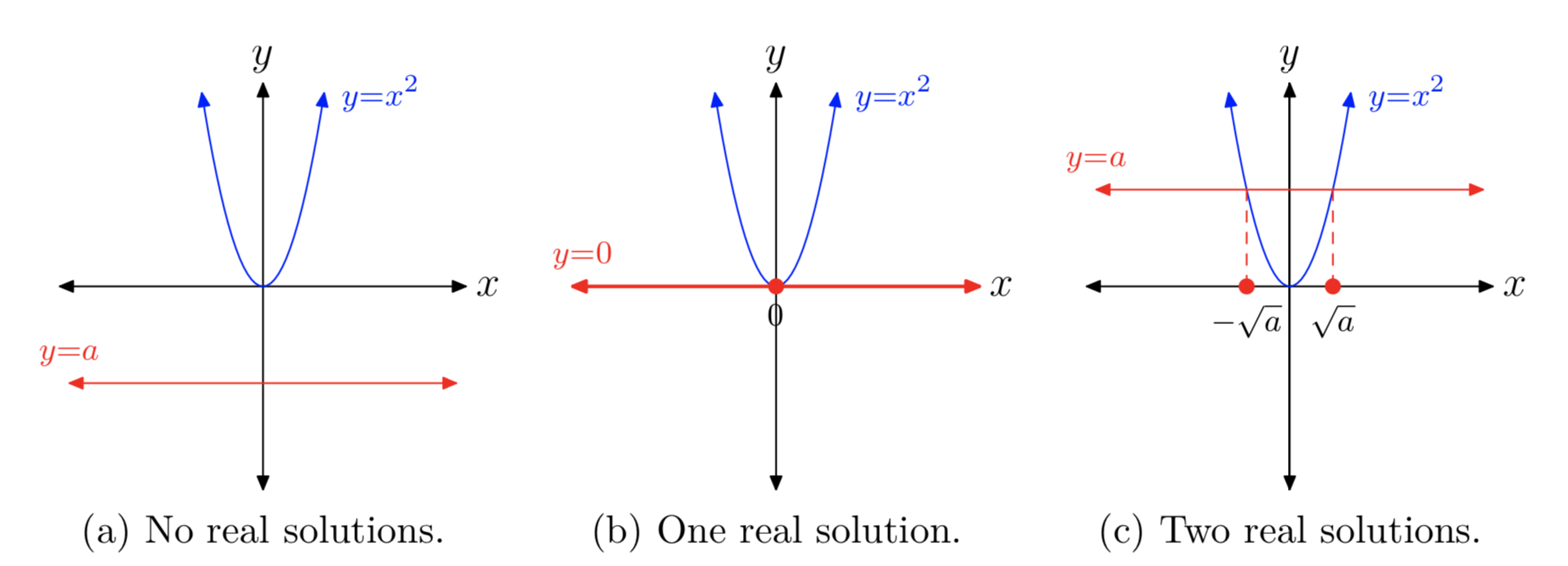
There are three cases, each depending on the value and sign of a. In each case, the graph of the left-hand side of \(x^2 = a\) is the parabola shown in Figures 1(a), (b), and (c).
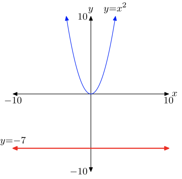
- Case I: a < 0
The graph of the right-hand side of \(x^2 = a\) is a horizontal line located a units below the x-axis. Hence, the graphs of \(y = x^2\) and y = a do not intersect and the equation \(x^2 = a\) has no real solutions. This case is shown in Figure 1(a). It follows that a negative number has no square root.
- Case II: a = 0
The graph of the right-hand side of \(x^2 = 0\) is a horizontal line that coincides with the x-axis. The graph of \(y = x^2\) intersects the graph of y = 0 at one point, at
the vertex of the parabola. Thus, the only solution of \(x^2 = 0\) is x = 0, as seen in Figure 2(b). The solution is the square root of 0, and is denoted \(\sqrt{0}\), so it follows \(\sqrt{0} = 0\).
- Case III: a > 0
The graph of the right-hand side of \(x^2 = a\) is a horizontal line located a units above the x-axis. The graphs of \(y = x^2\) and y = a have two points of intersection, and therefore the equation \(x^2 = a\) has two real solutions, as shown in Figure 1(c). The solutions of \(x^2 = a\) are \(x = \pm \sqrt{a}\). Note that we have two notations, one that calls for the positive solution and a second that calls for the negative solution.
Let’s look at some examples.
What are the solutions of \(x^2 = −5\)?
The graph of the left-hand side of \(x^2 = −5\) is the parabola depicted in Figure 1(a). The graph of the right-hand side of \(x^2 = −5\) is a horizontal line located 5 units below the x-axis. Thus, the graphs do not intersect and the equation \(x^2 = −5\) has no real solutions.
You can also reason as follows. We’re asked to find a solution of \(x^2 = −5\), so you must find a number whose square equals −5. However, whenever you square a real number, the result is always nonnegative (zero or positive). It is not possible to square a real number and get −5.
Note that this also means that it is not possible to take the square root of a negative number. That is, \(\sqrt{−5}\) is not a real number.
What are the solutions of \(x^2 = 0\)?
There is only one solution, namely x = 0. Note that this means that \(\sqrt{0} = 0\).
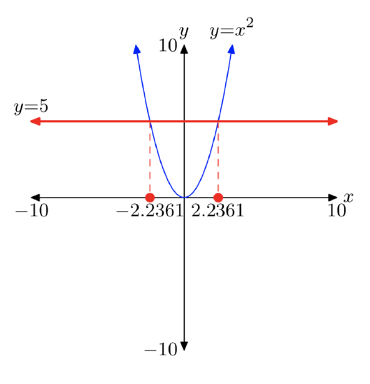
What are the solutions of \(x^2 = 25\)?
The graph of the left-hand side of \(x^2 = 25\) is the parabola depicted in Figure 1(c). The graph of the right-hand side of \(x^2 = 25\) is a horizontal line located 25 units above the x-axis. The graphs will intersect in two points, so the equation \(x^2 = 25\) has two real solutions.
The solutions of \(x^2 = 25\) are called square roots of 25 and are written \(x = \pm \sqrt{25}\). In this case, we can simplify further and write \(x = \pm 5\).
It is extremely important to note the symmetry in Figure 1(c) and note that we have two real solutions, one negative and one positive. Thus, we need two notations, one for the positive square root of 25 and one for the negative square root 25.
Note that \((5)^2 = 25\), so x = 5 is the positive solution of \(x^2 = 25\). For the positive solution, we use the notation
\(\sqrt{25} = 5\).
This is pronounced “the positive square root of 25 is 5.”
On the other hand, note that \((−5)^2 = 25\), so x = −5 is the negative solution of \(x^2 = 25\). For the negative solution, we use the notation
\(−\sqrt{25} = −5\).
This is pronounced “the negative square root of 25 is −5.”
This discussion leads to the following detailed summary.
The solutions of \(x^2 = a\) are called “square roots of a.”
- Case I: a < 0. The equation \(x^2 = a\) has no real solutions.
- Case II: a = 0. The equation \(x^2 = a\) has one real solution, namely x = 0. Thus, \(\sqrt{0} = 0\).
- Case III: a > 0. The equation \(x^2 = a\) has two real solutions, \(x = \pm \sqrt{a}\). The notation \(\sqrt{a}\) calls for the positive square root of a, that is, the positive solution of \(x^2 = a\). The notation \(−\sqrt{a}\) calls for the negative square root of a, that is, the negative solution of \(x^2 = a\).
Cube Roots: Let’s move on to the definition of cube roots.
Given a real number a, a “cube root of a” is a number x such that \(x^3 = a\).
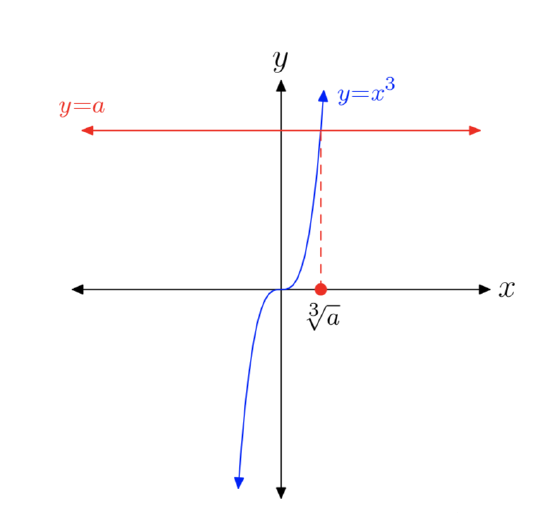
For example, 2 is a cube root of 8 since \(2^3 = 8\). Likewise, −4 is a cube root of −64 since \((−4)^3 = −64\). Thus, taking the cube root is the “opposite” of cubing, so the definition of cube root must be closely connected to the graph of \(y = x^3\), the cubing function. Therefore, we look for solutions of
\(x^3 = a\). (12)
Because of the shape of the graph of \(y = x^3\), there is only one case to consider. The graph of the left-hand side of \(x^3 = a\) is shown in Figure 2. The graph of the right-hand side of \(x^3 = a\) is a horizontal line, located a units above, on, or below the x-axis, depending on the sign and value of a. Regardless of the location of the horizontal line y = a, there will only be one point of intersection, as shown in Figure 2.
A detailed summary of cube roots follows.
The solutions of \(x^3 = a\) are called the “cube roots of a.” Whether a is negative, zero, or positive makes no difference. There is exactly one real solution, namely \(x = \sqrt[3]{a}\).
Let’s look at some examples.
What are the solutions of \(x^3 = 8\)?
The graph of the left-hand side of \(x^3 = 8\) is the cubic polynomial shown in Figure 2. The graph of the right-hand side of \(x^3 = 8\) is a horizontal line located 8 units above the x-axis. The graphs have one point of intersection, so the equation \(x^3 = 8\) has exactly one real solution.
The solutions of \(x^3 = 8\) are called “cube roots of 8.” As shown from the graph, there is exactly one real solution of \(x^3 = 8\), namely \(x = \sqrt[3]{8}\). Now since \((2)^3 = 8\), it follows that x = 2 is a real solution of \(x^3 = 8\). Consequently, the cube root of 8 is 2, and we write
\(\sqrt[3]{8} = 2\).
Note that in the case of cube root, there is no need for the two notations we saw in the square root case (one for the positive square root, one for the negative square root). This is because there is only one real cube root. Thus, the notation \(\sqrt[3]{8}\) is pronounced “the cube root of 8.”
What are the solutions of \(x^3 = 0\)?
There is only one solution of \(x^3 = 0\), namely x = 0. This means that \(\sqrt[3]{0} = 0\).
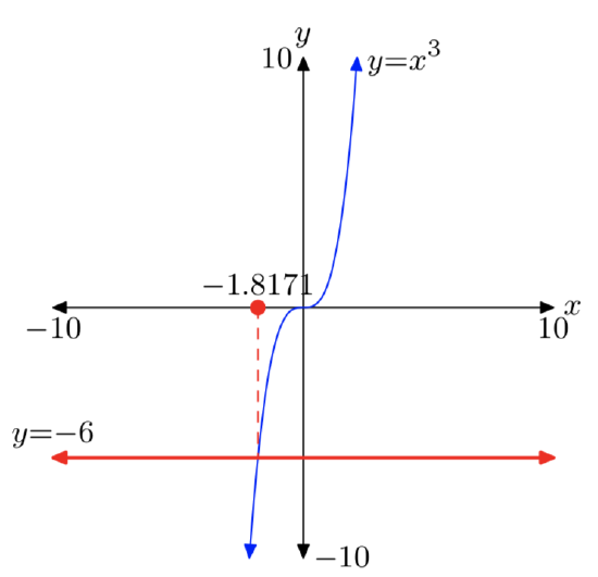
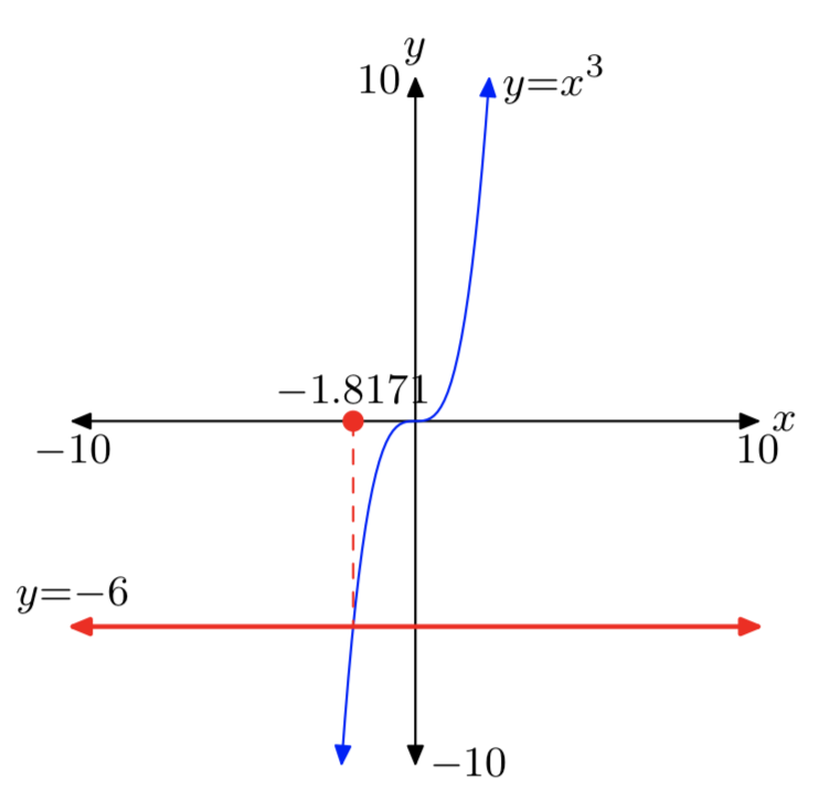
What are the solutions of \(x^3 = −8\)?
The graph of the left-hand side of \(x^3 = −8\) is the cubic polynomial shown in Figure 2. The graph of the right-hand side of \(x^3 = −8\) is a horizontal line located 8 units below the x-axis. The graphs have only one point of intersection, so the equation \(x^3 = −8\) has exactly one real solution, denoted \(x = \sqrt[3]{−8}\). Now since \((−2)^3 = −8\), it follows that x = −2 is a real solution of \(x^3 = −8\). Consequently, the cube root of −8 is −2, and we write
\(\sqrt[3]{−8} = −2\).
Again, because there is only one real solution of \(x^3 = −8\), the notation \(\sqrt[3]{−8}\) is pronounced “the cube root of −8.” Note that, unlike the square root of a negative number, the cube root of a negative number is allowed.
Higher Roots: The previous discussions generalize easily to higher roots, such as fourth roots, fifth roots, sixth roots, etc.
Given a real number a and a positive integer n, an “\(n^{th}\) root of a” is a number x such that \(x^n = a\).
For example, 2 is a \(6^{th}\) root of 64 since \(2^6 = 64\) and −3 is a fifth root of −243 since \((−3)^5 = −243\).
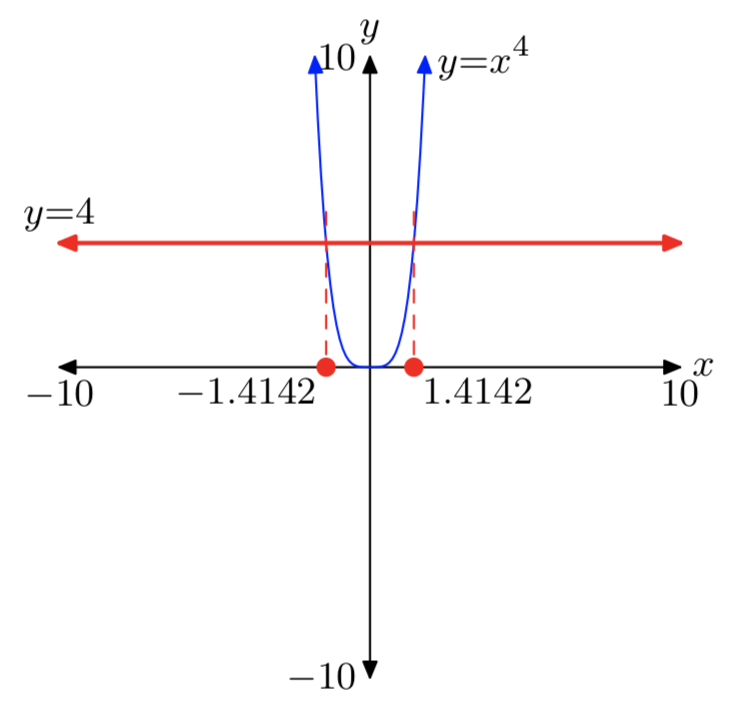
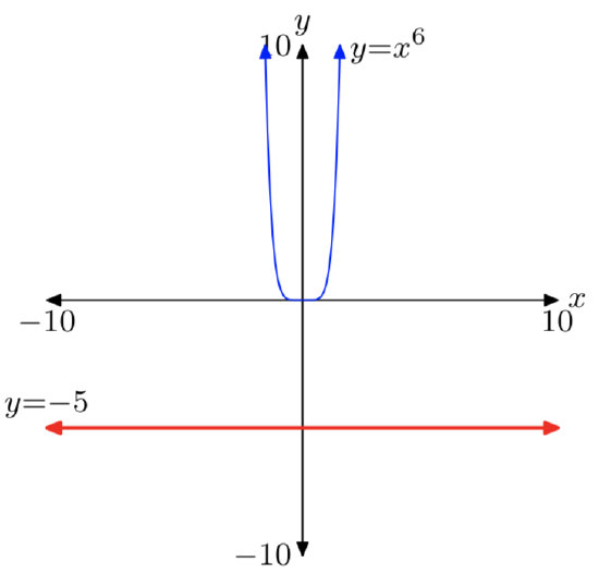
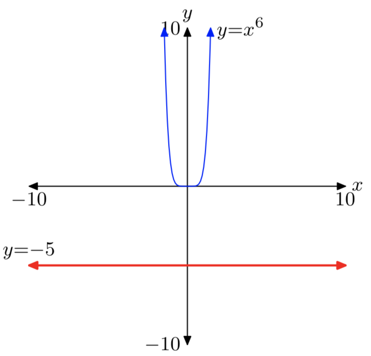
The case of even roots (i.e., when n is even) closely parallels the case of square roots. That’s because when the exponent n is even, the graph of \(y = x^n\) closely resembles that of \(y = x^2\). For example, observe the case for fourth roots shown in Figures 3(a), (b), and (c).
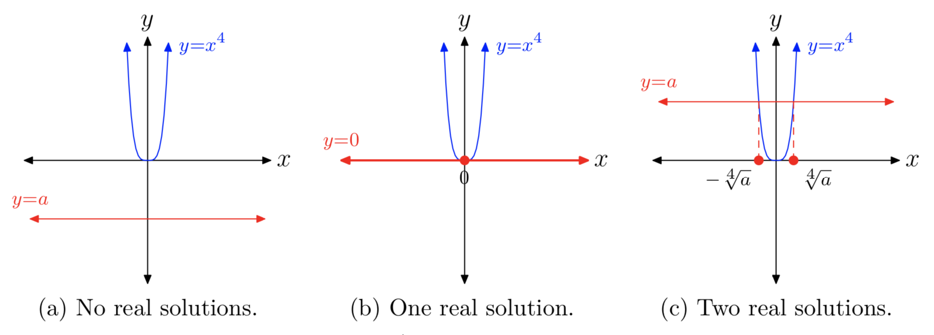
The discussion for even \(n^{th}\) roots closely parallels that presented in the introduction of square roots, so without further ado, we go straight to the summary.
If n is a positive even integer, then the solutions of \(x^n = a\) are called “\(n^{th}\) roots of a.”
- Case I: a < 0. The equation \(x^n = a\) has no real solutions.
- Case II: a = 0. The equation \(x^n = a\) has exactly one real solution, namely x = 0. Thus, \(\sqrt[n]{0} = 0\).
- Case III: a > 0. The equation \(x^n =a\) has two real solutions, \(x = \pm \sqrt[n]{a}\). The notation \(\sqrt[n]{a}\) calls for the positive \(n^{th}\) root of a, that is, the positive solution of \(x^n = a\). The notation \(−\sqrt[n]{a}\) calls for the negative \(n^{th}\) root of a, that is, the negative solution of \(x^n = a\).
Likewise, the case of odd roots (i.e., when n is odd) closely parallels the case of cube roots. That’s because when the exponent n is odd, the graph of \(y = x^n\) closely resembles that of \(y = x^3\). For example, observe the case for fifth roots shown in Figure 4.
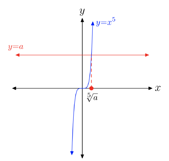
The discussion of odd \(n^{th}\) roots closely parallels the introduction of cube roots which we discussed earlier. So, without further ado, we proceed straight to the summary.
If n is a positive odd integer, then the solutions of \(x^n = a\) are called the “\(n^{th}\) roots of a.” Whether a is negative, zero, or positive makes no difference. There is exactly one real solution of \(x^n = a\), denoted \(x = \sqrt[n]{a}\).
Remark 17. The symbols \(\sqrt{}\) and \(\sqrt[n]{}\) for square root and \(n^{th}\) root, respectively, are also called radicals.
We’ll close this section with a few more examples.
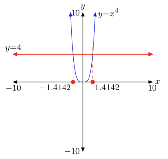
What are the solutions of \(x^4 = 16\)?
The graph of the left-hand side of \(x^4 = 16\) is the quartic polynomial shown in Figure 3(c). The graph of the right-hand side of \(x^4 = 16\) is a horizontal line, located 16 units above the x-axis. The graphs will intersect in two points, so the equation \(x^4 = 16\) has two real solutions.
The solutions of \(x^4 = 16\) are called fourth roots of 16 and are written \(x = \pm \sqrt[4]{16}\). It is extremely important to note the symmetry in Figure 3(c) and note that we have two real solutions of \(x^4 = 16\), one of which is negative and the other positive. Hence, we need two notations, one for the positive fourth root of 16 and one for the negative fourth root of 16.
Note that \(2^4 = 16\), so x = 2 is the positive real solution of \(x^4 = 16\). For this positive solution, we use the notation
\(\sqrt[4]{16} = 2\).
This is pronounced “the positive fourth root of 16 is 2.”
On the other hand, note that \((−2)^4 = 16\), so x = −2 is the negative real solution of \(x^4 = 16\). For this negative solution, we use the notation
\(−\sqrt[4]{16} = −2\). (19)
This is pronounced “the negative fourth root of 16 is −2.”
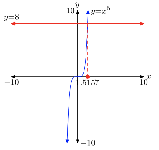
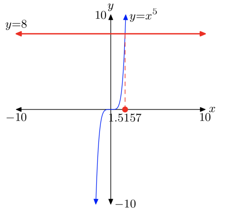
What are the solutions of \(x^5 = −32\)?
The graph of the left-hand side of \(x^5 = −32\) is the quintic polynomial pictured in Figure 4. The graph of the right-hand side of \(x^5 = −32\) is a horizontal line, located 32 units below the x-axis. The graphs have one point of intersection, so the equation \(x^5 = −32\) has exactly one real solution.
The solutions of \(x^5 = −32\) are called “fifth roots of −32.” As shown from the graph, there is exactly one real solution of \(x^5 = −32\), namely \(x = \sqrt[5]{−32}\). Now since \((−2)^5 = −32\), it follows that x = −2 is a solution of \(x^5 = −32\). Consequently, the fifth root of −32 is −2, and we write
\(\sqrt[5]{−32} = −2\).
Because there is only one real solution, the notation \(\sqrt[5]{−32}\) is pronounced “the fifth root of −32.” Again, unlike the square root or fourth root of a negative number, the fifth root of a negative number is allowed.
Not all roots simplify to rational numbers. If that were the case, it would not even be necessary to implement radical notation. Consider the following example.
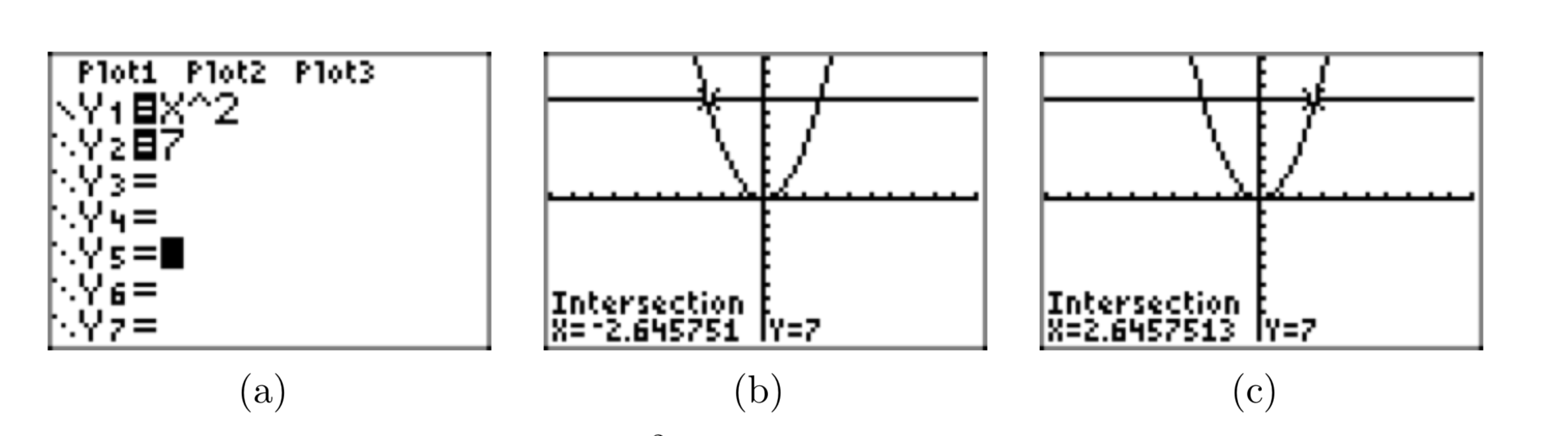
Find all real solutions of the equation \(x^2 = 7\), both graphically and algebraically, and compare your results.
We could easily sketch rough graphs of \(y = x^2\) and y = 7 by hand, but let’s seek a higher level of accuracy by asking the graphing calculator to handle this task.
- Load the equation \(y = x^2\) and y = 7 into Y1 and Y2 in the calculator’s Y= menu, respectively. This is shown in Figure 5(a).
- Use the intersect utility on the graphing calculator to find the coordinates of the points of intersection. The x-coordinates of these points, shown in Figure 5(b) and (c), are the solutions to the equation \(x^2 = 7\).
Guidelines for Reporting Graphing Calculator Solutions. Recall the standard method for reporting graphing calculator results on your homework:
- Copy the image from your viewing window onto your homework paper. Label and scale each axis with xmin, xmax, ymin, and ymax, then label each graph with its equation, as shown in Figure 6.
- Drop dashed vertical lines from each point of intersection to the x-axis. Shade and label your solutions on the x-axis.
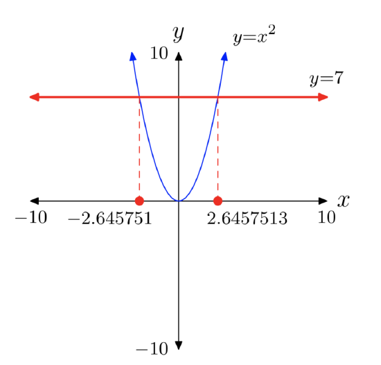
Hence, the approximate solutions are \(x \approx −2.645751\) or \(x \approx 2.6457513\).
On the other hand, to find analytic solutions of \(x^2 = 7\), we simply take plus or minus the square root of 7.
\(x^2 = 7\)
\(\sqrt{x} = \pm 7\)
To compare these exact solutions with the approximate solutions found by using the graphing calculator, use a calculator to compute \(\pm \sqrt{7}\), as shown in Figure 7.
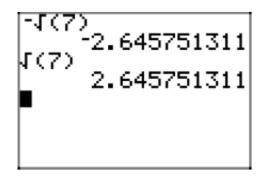
Note that these approximations of \(−\sqrt{7}\) and \(\sqrt{7}\) agree quite nicely with the solutions found using the graphing calculator’s intersect utility and reported in Figure 6.
Both \(−\sqrt{7}\) and \(\sqrt{7}\) are examples of irrational numbers, that is, numbers that cannot be expressed in the form \(\frac{p}{q}\), where p and q are integers.
Rational Exponents
As with the definition of negative and zero exponents, discussed earlier in this section, it turns out that rational exponents can be defined in such a way that the Laws of Exponents will still apply (and in fact, there’s only one way to do it).
The third law gives us a hint on how to define rational exponents. For example, suppose that we want to define \(2^{\frac{1}{3}}\). Then by the third law,
\((2^{\frac{1}{3}})^3 = 2^{\frac{1}{3} \cdot 3} = 2^1 = 2\),
so, by taking cube roots of both sides, we must define \(2^{\frac{1}{3}}\). by the formula
\(2^{\frac{1}{3}} = \sqrt[3]{2}\).
The same argument shows that if n is any odd positive integer, then \(2^{\frac{1}{n}}\) must be defined by the formula
\(2^{\frac{1}{n}} = \sqrt[n]{2}\).
However, for an even integer n, there appears to be a choice. Suppose that we want to define \(2^{\frac{1}{2}}\). Then
\((2^{\frac{1}{2}})^2 = 2^{\frac{1}{2} \cdot 2} = 2^1 = 2\),
so,
\(2^{\frac{1}{2}} = \sqrt{2}\).
However, the negative choice for the exponent \(\frac{1}{2}\) leads to problems, because then certain expressions are not defined. For example, it would follow from the third law that
\((2^{\frac{1}{2}})^\frac{1}{2} = −\sqrt{−\sqrt{2}}\).
But \(−\sqrt{2}\) is negative, so \(\sqrt{−\sqrt{2}}\) is not defined. Therefore, it only makes sense to use the positive choice. Thus, for all n, even and odd, \(2^{\frac{1}{n}}\) is defined by the formula
\(2^{\frac{1}{n}} = \sqrt[n]{2}\).
In a similar manner, for a general positive rational \(\frac{m}{n}\) the third law implies that
\(2^{\frac{m}{n}} = (2^m)^{\frac{1}{n}} = \sqrt[n]{2^m}\)
But also,
\(2^{\frac{m}{n}} = (2^{\frac{1}{n}})^m = (\sqrt[n]{2})^m\)
Thus,
\(2^{\frac{m}{n}} = \sqrt[n]{2^m} = (\sqrt[n]{2})^m\)
Finally, negative rational exponents are defined in the usual manner for negative exponents:
\(2^{−\frac{m}{n}} = \frac{1}{2^{\frac{m}{n}}}\)
More generally, here is the final general definition. With this definition, the Laws of Exponents hold for all rational exponents.
For a positive rational exponent \(\frac{m}{n}\), and b > 0
\(b^{\frac{m}{n}} = \sqrt[n]{b^m} = (\sqrt[n]{b})^m\) (23)
For a negative rational exponent \(−\frac{m}{n}\),
\(b^{−\frac{m}{n}} = \frac{1}{b^{\frac{m}{n}}}\) (24)
Remark 25. For b < 0, the same definitions make sense only when n is odd. For example \((−2)^{\frac{1}{4}}\) is not defined.
Compute the exact values of
(a) \(4^{\frac{5}{2}}\)
(b) \(64^{\frac{2}{3}}\)
(c) \(81^{−\frac{3}{4}}\)
- Answer
-
(a) \(4^{\frac{5}{2}} = (4^{\frac{1}{2}})^5 = (\sqrt{4})^5 = 2^5 = 32\)
(b) \(64^{\frac{2}{3}} = (64^\frac{1}{3})^2 = (\sqrt[3]{64})^2 = 4^2 = 16\)
(c) \(81^{−\frac{3}{4}} = \frac{1}{81^{\frac{3}{4}}} = \frac{1}{(81^{\frac{1}{4}})^3} = \frac{1}{3^3} = \frac{1}{27}\)
Simplify the following expressions, and write them in the form \(x^r\):
(a) \(x^{\frac{2}{3}}x^{\frac{1}{4}}\)
(b) \(\frac{x^{\frac{2}{3}}}{x^{\frac{1}{4}}}\)
(c) \((x^{−\frac{2}{3}})^{\frac{1}{4}}\)
- Answer
-
(a) \(x^{\frac{2}{3}}x^{\frac{1}{4}} = x^{\frac{2}{3}+\frac{1}{4}} = x^{\frac{11}{12}}\)
(b) \(\frac{x^{\frac{2}{3}}}{x^{\frac{1}{4}}} = x^{\frac{2}{3}−\frac{1}{4}} = x^{\frac{5}{12}}\)
(c) \((x^{−\frac{2}{3}})^{\frac{1}{4}} = x^{−\frac{2}{3} \cdot \frac{1}{4}} = x^{−\frac{1}{6}}\)
Use rational exponents to simplify \(\sqrt[5]{\sqrt{x}}\), and write it as a single radical.
- Answer
-
\(\sqrt[5]{\sqrt{x}} = (\sqrt{x})^{\frac{1}{5}} = (x^{\frac{1}{2}})^{\frac{1}{5}} = (x^{\frac{1}{2} \cdot \frac{1}{5}} = x^{\frac{1}{10}} = \sqrt[10]{x}\)
Use a calculator to approximate \(2^{\frac{5}{8}}\).
- Answer
-
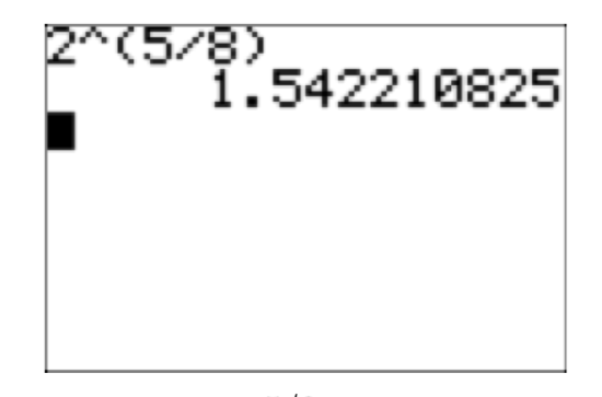
Figure 8. \(2^{\frac{5}{8}} \approx 1.542210825\)
Irrational Exponents
What about irrational exponents? Is there a way to define numbers like \(2^{\sqrt{2}}\) and \(3^{\pi}\)? It turns out that the answer is yes. While a rigorous definition of \(b^s\) when s is irrational is beyond the scope of this book, it’s not hard to see how one could proceed to find a value for such a number. For example, if we want to compute the value of \(2^{\sqrt{2}}\), we can start with rational approximations for \(\sqrt{2}\). Since \(\sqrt{2}\) = 1.41421356237310 . . ., the successive powers
\(2^1\), \(2^{1.4}\), \(2^{1.41}\), \(2^{1.414}\), \(2^{1.4142}\), \(2^{1.41421}\), \(2^{1.414213}\), \(2^{1.4142135}\), \(2^{1.41421356}\), \(2^{1.414213562}\), \(2^{1.4142135623}\), . . .
should be closer and closer approximations to the desired value of \(2^{\sqrt{2}}\).
In fact, using more advanced mathematical theory (ultimately based on the actual construction of the real number system), it can be shown that these powers approach a single real number, and we define \(2^{\sqrt{2}}\) to be that number. Using your calculator, you can observe this convergence and obtain an approximation by computing the powers above.
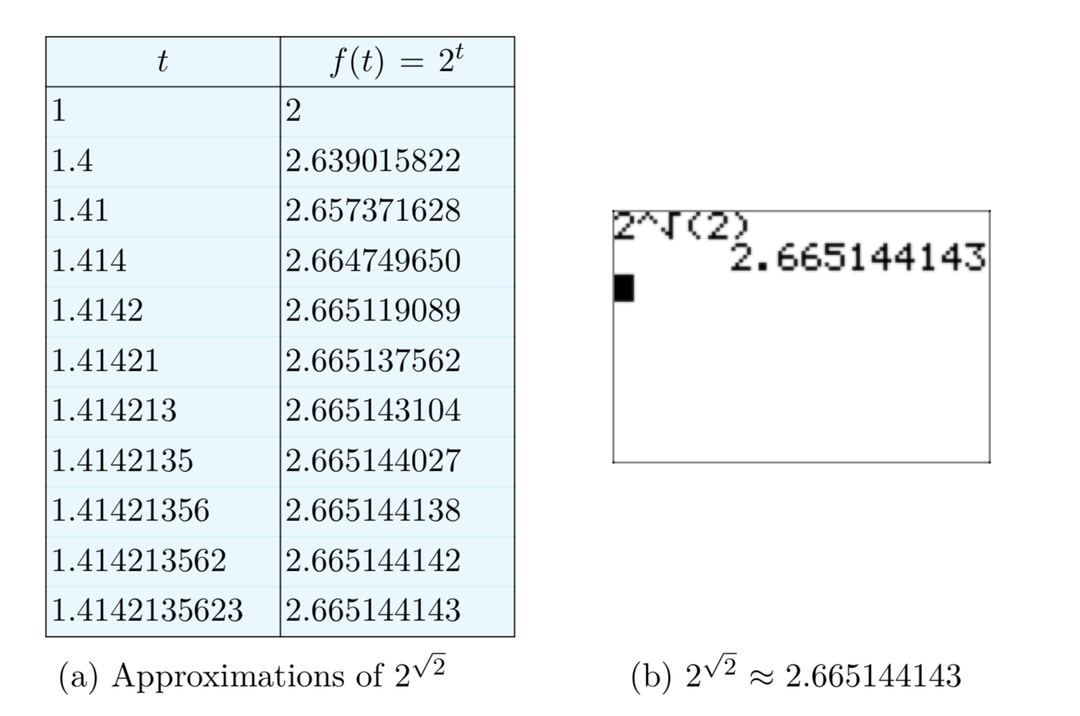
The last value in the table in Figure 9(a) is a correct approximation of \(2^{\sqrt{2}}\) to 10 digits of accuracy. Your calculator will obtain this same approximation when you ask it to compute \(2^{\sqrt{2}}\) directly (see Figure 9(b)).
In a similar manner, \(b^s\) can be defined for any irrational exponent s and any b > 0. Combined with the earlier work in this section, it follows that \(b^s\) is defined for every real exponent s.
Exercise
In Exercises 1-12, compute the exact value.
\(3^{−5}\)
- Answer
-
\(\frac{1}{243}\)
\(4^2\)
\((\frac{3}{2})^3\)
- Answer
-
\(\frac{27}{8}\)
\((\frac{2}{3})^1\)
\(6^{−2}\)
- Answer
-
\(\frac{1}{36}\)
\(4^{−3}\)
\((\frac{2}{3})^{−3}\)
- Answer
-
\(\frac{27}{8}\)
\((\frac{1}{3})^{−3}\)
\(7^1\)
- Answer
-
7
\((\frac{3}{2})^{−4}\)
\((\frac{5}{6})^3\)
- Answer
-
\(\frac{125}{216}\)
\(3^2\)
In Exercises 13-24, perform each of the following tasks for the given equation.
- Load the left- and right-hand sides of the given equation into Y1 and Y2, respectively. Adjust the WINDOW parameters until all points of intersection (if any) are visible in your viewing window. Use the intersect utility in the CALC menu to determine the coordinates of any points of intersection.
- Make a copy of the image in your viewing window on your homework paper. Label and scale each axis with xmin, xmax, ymin, and ymax. Label each graph with its equation. Drop dashed vertical lines from each point of intersection to the x-axis, then shade and label each solution of the given equation on the x-axis. Remember to draw all lines with a ruler.
- Solve each problem algebraically. Use a calculator to approximate any radicals and compare these solutions with those found in parts (1) and (2).
\(x^2 = 5\)
- Answer
-
\(x = \pm \sqrt{5}\)

\(x^2 = 7\)
\(x^2 = −7\)
- Answer
-
No real solutions.

\(x^2 = −3\)
\(x^3 = −6\)
- Answer
-
\(x = \sqrt[3]{−6}\)
\(x^3 = −4\)
\(x^4 = 4\)
- Answer
-
\(x = \pm \sqrt[4]{4}\)
\(x^4 = −7\)
\(x^5 = 8\)
- Answer
-
\(x = \sqrt[5]{8}\)
\(x^5 = 4\)
\(x^6 = −5\)
- Answer
-
No real solutions.
\(x^6 = 9\)
In Exercises 25-40, simplify the given radical expression.
\(\sqrt{49}\)
- Answer
-
7
\(\sqrt{121}\)
\(\sqrt{−36}\)
- Answer
-
Not a real number.
\(\sqrt{−100}\)
\(\sqrt[3]{−1}\)
- Answer
-
3
\(\sqrt[3]{−1}\)
\(\sqrt[3]{−125}\)
- Answer
-
−5
\(\sqrt[3]{64}\)
\(\sqrt[4]{−16}\)
- Answer
-
Not a real number.
\(\sqrt[4]{81}\)
\(\sqrt[4]{16}\)
- Answer
-
2
\(\sqrt[3]{−625}\)
\(\sqrt[5]{−32}\)
- Answer
-
−2
\(\sqrt[5]{243}\)
\(\sqrt[5]{1024}\)
- Answer
-
4
\(\sqrt[5]{−3125}\)
Compare and contrast \(\sqrt{(−2)^2}\) and \((\sqrt{−2})^2\).
- Answer
-
\(\sqrt{(−2)^2} = 2\), while \((\sqrt{−2})^2\) is not a real number.
Compare and contrast \(\sqrt[4]{(−3)^4}\) and \((\sqrt[4]{−3})^4\).
Compare and contrast \(\sqrt[3]{(−5)^3}\) and \((\sqrt[3]{−5})^3\).
- Answer
-
Both equal −5.
Compare and contrast \(\sqrt[5]{(−2)^5}\) and \((\sqrt[5]{−2})^5\).
In Exercises 45-56, compute the exact value.
\(25^{−\frac{3}{2}}\)
- Answer
-
\(\frac{1}{125}\)
\(16^{−\frac{5}{4}}\)
\(8^{\frac{4}{3}}\)
- Answer
-
16
\(625^{−\frac{3}{4}}\)
\(16^{\frac{3}{2}}\)
- Answer
-
64
\(64^{\frac{2}{3}}\)
\(27^{\frac{2}{3}}\)
- Answer
-
9
\(625^{\frac{3}{4}}\)
\(256^{\frac{5}{4}}\)
- Answer
-
1024
\(4^{−\frac{3}{2}}\)
\(256^{−\frac{3}{4}}\)
- Answer
-
\(\frac{1}{64}\)
\(81^{−\frac{5}{4}}\)
In Exercises 57-64, simplify the product, and write your answer in the form \(x^r\).
\(x^{\frac{5}{4}}x^{\frac{5}{4}}\)
- Answer
-
\(x^{\frac{5}{2}}\)
\(x^{\frac{5}{3}}x^{−\frac{5}{4}}\)
\(x^{−\frac{1}{3}}x^{\frac{5}{2}}\)
- Answer
-
\(x^{\frac{13}{6}}\)
\(x^{−\frac{3}{5}}x^{\frac{3}{2}}\)
\(x^{\frac{4}{5}}x^{−\frac{4}{3}}\)
- Answer
-
\(x^{−\frac{8}{15}}\)
\(x^{−\frac{5}{4}}x^{\frac{1}{2}}\)
\(x^{−\frac{2}{5}}x^{−\frac{3}{2}}\)
- Answer
-
\(x^{−\frac{19}{10}}\)
\(x^{−\frac{5}{4}}x^{\frac{5}{2}}\)
In Exercises 65-72, simplify the quotient, and write your answer in the form \(x^r\).
\(\frac{x^{−\frac{5}{4}}}{x^{\frac{1}{5}}}\)
- Answer
-
\(x^{−\frac{29}{20}}\)
\(\frac{x^{−\frac{2}{3}}}{x^{\frac{1}{4}}}\)
\(\frac{x^{−\frac{1}{2}}}{x^{−\frac{3}{5}}}\)
- Answer
-
\(x^{\frac{1}{10}}\)
\(\frac{x^{−\frac{5}{2}}}{x^{\frac{5}{2}}}\)
\(\frac{x^{\frac{3}{5}}}{x^{−\frac{1}{4}}}\)
- Answer
-
\(x^{\frac{17}{20}}\)
\(\frac{x^{\frac{1}{3}}}{x^{−\frac{1}{2}}}\)
\(\frac{x^{−\frac{5}{4}}}{x^{\frac{2}{3}}}\)
- Answer
-
\(x^{−\frac{23}{12}}\)
\(\frac{x^{\frac{1}{3}}}{x^{\frac{1}{2}}}\)
In Exercises 73-80, simplify the expression, and write your answer in the form \(x^r\).
\((x^{\frac{1}{2}})^{\frac{4}{3}}\)
- Answer
-
\(x^{\frac{2}{3}}\)
\((x^{−\frac{1}{2}})^{−\frac{1}{2}}\)
\((x^{−\frac{5}{4}})^{\frac{1}{2}}\)
- Answer
-
\(x^{−\frac{5}{8}}\)
\((x^{−\frac{1}{5}})^{−\frac{3}{2}}\)
\((x^{−\frac{1}{2}})^{\frac{3}{2}}\)
- Answer
-
\(x^{−\frac{3}{4}}\)
\((x^{−\frac{1}{3}})^{−\frac{1}{2}}\)
\((x^{\frac{1}{5}})^{−\frac{1}{2}}\)
- Answer
-
\(x^{−\frac{1}{10}}\)
\((x^{\frac{2}{5}})^{−\frac{1}{5}}\)