4.2: Solve Systems of Linear Equations with Two Variables
- Page ID
- 5138
\( \newcommand{\vecs}[1]{\overset { \scriptstyle \rightharpoonup} {\mathbf{#1}} } \)
\( \newcommand{\vecd}[1]{\overset{-\!-\!\rightharpoonup}{\vphantom{a}\smash {#1}}} \)
\( \newcommand{\dsum}{\displaystyle\sum\limits} \)
\( \newcommand{\dint}{\displaystyle\int\limits} \)
\( \newcommand{\dlim}{\displaystyle\lim\limits} \)
\( \newcommand{\id}{\mathrm{id}}\) \( \newcommand{\Span}{\mathrm{span}}\)
( \newcommand{\kernel}{\mathrm{null}\,}\) \( \newcommand{\range}{\mathrm{range}\,}\)
\( \newcommand{\RealPart}{\mathrm{Re}}\) \( \newcommand{\ImaginaryPart}{\mathrm{Im}}\)
\( \newcommand{\Argument}{\mathrm{Arg}}\) \( \newcommand{\norm}[1]{\| #1 \|}\)
\( \newcommand{\inner}[2]{\langle #1, #2 \rangle}\)
\( \newcommand{\Span}{\mathrm{span}}\)
\( \newcommand{\id}{\mathrm{id}}\)
\( \newcommand{\Span}{\mathrm{span}}\)
\( \newcommand{\kernel}{\mathrm{null}\,}\)
\( \newcommand{\range}{\mathrm{range}\,}\)
\( \newcommand{\RealPart}{\mathrm{Re}}\)
\( \newcommand{\ImaginaryPart}{\mathrm{Im}}\)
\( \newcommand{\Argument}{\mathrm{Arg}}\)
\( \newcommand{\norm}[1]{\| #1 \|}\)
\( \newcommand{\inner}[2]{\langle #1, #2 \rangle}\)
\( \newcommand{\Span}{\mathrm{span}}\) \( \newcommand{\AA}{\unicode[.8,0]{x212B}}\)
\( \newcommand{\vectorA}[1]{\vec{#1}} % arrow\)
\( \newcommand{\vectorAt}[1]{\vec{\text{#1}}} % arrow\)
\( \newcommand{\vectorB}[1]{\overset { \scriptstyle \rightharpoonup} {\mathbf{#1}} } \)
\( \newcommand{\vectorC}[1]{\textbf{#1}} \)
\( \newcommand{\vectorD}[1]{\overrightarrow{#1}} \)
\( \newcommand{\vectorDt}[1]{\overrightarrow{\text{#1}}} \)
\( \newcommand{\vectE}[1]{\overset{-\!-\!\rightharpoonup}{\vphantom{a}\smash{\mathbf {#1}}}} \)
\( \newcommand{\vecs}[1]{\overset { \scriptstyle \rightharpoonup} {\mathbf{#1}} } \)
\(\newcommand{\longvect}{\overrightarrow}\)
\( \newcommand{\vecd}[1]{\overset{-\!-\!\rightharpoonup}{\vphantom{a}\smash {#1}}} \)
\(\newcommand{\avec}{\mathbf a}\) \(\newcommand{\bvec}{\mathbf b}\) \(\newcommand{\cvec}{\mathbf c}\) \(\newcommand{\dvec}{\mathbf d}\) \(\newcommand{\dtil}{\widetilde{\mathbf d}}\) \(\newcommand{\evec}{\mathbf e}\) \(\newcommand{\fvec}{\mathbf f}\) \(\newcommand{\nvec}{\mathbf n}\) \(\newcommand{\pvec}{\mathbf p}\) \(\newcommand{\qvec}{\mathbf q}\) \(\newcommand{\svec}{\mathbf s}\) \(\newcommand{\tvec}{\mathbf t}\) \(\newcommand{\uvec}{\mathbf u}\) \(\newcommand{\vvec}{\mathbf v}\) \(\newcommand{\wvec}{\mathbf w}\) \(\newcommand{\xvec}{\mathbf x}\) \(\newcommand{\yvec}{\mathbf y}\) \(\newcommand{\zvec}{\mathbf z}\) \(\newcommand{\rvec}{\mathbf r}\) \(\newcommand{\mvec}{\mathbf m}\) \(\newcommand{\zerovec}{\mathbf 0}\) \(\newcommand{\onevec}{\mathbf 1}\) \(\newcommand{\real}{\mathbb R}\) \(\newcommand{\twovec}[2]{\left[\begin{array}{r}#1 \\ #2 \end{array}\right]}\) \(\newcommand{\ctwovec}[2]{\left[\begin{array}{c}#1 \\ #2 \end{array}\right]}\) \(\newcommand{\threevec}[3]{\left[\begin{array}{r}#1 \\ #2 \\ #3 \end{array}\right]}\) \(\newcommand{\cthreevec}[3]{\left[\begin{array}{c}#1 \\ #2 \\ #3 \end{array}\right]}\) \(\newcommand{\fourvec}[4]{\left[\begin{array}{r}#1 \\ #2 \\ #3 \\ #4 \end{array}\right]}\) \(\newcommand{\cfourvec}[4]{\left[\begin{array}{c}#1 \\ #2 \\ #3 \\ #4 \end{array}\right]}\) \(\newcommand{\fivevec}[5]{\left[\begin{array}{r}#1 \\ #2 \\ #3 \\ #4 \\ #5 \\ \end{array}\right]}\) \(\newcommand{\cfivevec}[5]{\left[\begin{array}{c}#1 \\ #2 \\ #3 \\ #4 \\ #5 \\ \end{array}\right]}\) \(\newcommand{\mattwo}[4]{\left[\begin{array}{rr}#1 \amp #2 \\ #3 \amp #4 \\ \end{array}\right]}\) \(\newcommand{\laspan}[1]{\text{Span}\{#1\}}\) \(\newcommand{\bcal}{\cal B}\) \(\newcommand{\ccal}{\cal C}\) \(\newcommand{\scal}{\cal S}\) \(\newcommand{\wcal}{\cal W}\) \(\newcommand{\ecal}{\cal E}\) \(\newcommand{\coords}[2]{\left\{#1\right\}_{#2}}\) \(\newcommand{\gray}[1]{\color{gray}{#1}}\) \(\newcommand{\lgray}[1]{\color{lightgray}{#1}}\) \(\newcommand{\rank}{\operatorname{rank}}\) \(\newcommand{\row}{\text{Row}}\) \(\newcommand{\col}{\text{Col}}\) \(\renewcommand{\row}{\text{Row}}\) \(\newcommand{\nul}{\text{Nul}}\) \(\newcommand{\var}{\text{Var}}\) \(\newcommand{\corr}{\text{corr}}\) \(\newcommand{\len}[1]{\left|#1\right|}\) \(\newcommand{\bbar}{\overline{\bvec}}\) \(\newcommand{\bhat}{\widehat{\bvec}}\) \(\newcommand{\bperp}{\bvec^\perp}\) \(\newcommand{\xhat}{\widehat{\xvec}}\) \(\newcommand{\vhat}{\widehat{\vvec}}\) \(\newcommand{\uhat}{\widehat{\uvec}}\) \(\newcommand{\what}{\widehat{\wvec}}\) \(\newcommand{\Sighat}{\widehat{\Sigma}}\) \(\newcommand{\lt}{<}\) \(\newcommand{\gt}{>}\) \(\newcommand{\amp}{&}\) \(\definecolor{fillinmathshade}{gray}{0.9}\)By the end of this section, you will be able to:
- Determine whether an ordered pair is a solution of a system of equations
- Solve a system of linear equations by graphing
- Solve a system of equations by substitution
- Solve a system of equations by elimination
- Choose the most convenient method to solve a system of linear equations
Before you get started, take this readiness quiz.
- For the equation \(y=\frac{2}{3}x−4\),
ⓐ Is \((6,0)\) a solution? ⓑ Is \((−3,−2)\) a solution?
If you missed this problem, review [link]. - Find the slope and y-intercept of the line \(3x−y=12\).
If you missed this problem, review [link]. - Find the x- and y-intercepts of the line \(2x−3y=12\).
If you missed this problem, review [link].
Determine Whether an Ordered Pair is a Solution of a System of Equations
In Solving Linear Equations, we learned how to solve linear equations with one variable. Now we will work with two or more linear equations grouped together, which is known as a system of linear equations.
When two or more linear equations are grouped together, they form a system of linear equations.
In this section, we will focus our work on systems of two linear equations in two unknowns. We will solve larger systems of equations later in this chapter.
An example of a system of two linear equations is shown below. We use a brace to show the two equations are grouped together to form a system of equations.
\[ \left\{ \begin{aligned} 2x+y & = 7 \\ x−2y & = 6 \end{aligned} \right. \nonumber \]
A linear equation in two variables, such as \(2x+y=7\), has an infinite number of solutions. Its graph is a line. Remember, every point on the line is a solution to the equation and every solution to the equation is a point on the line.
To solve a system of two linear equations, we want to find the values of the variables that are solutions to both equations. In other words, we are looking for the ordered pairs \((x,y)\) that make both equations true. These are called the solutions of a system of equations.
The solutions of a system of equations are the values of the variables that make all the equations true. A solution of a system of two linear equations is represented by an ordered pair \((x,y)\).
To determine if an ordered pair is a solution to a system of two equations, we substitute the values of the variables into each equation. If the ordered pair makes both equations true, it is a solution to the system.
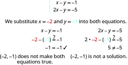
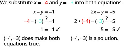
Determine whether the ordered pair is a solution to the system \(\left \{ \begin{array} {l} x−y = −1 \\ 2x−y = −5 \end{array} \right. \).
ⓐ \((−2,−1)\) ⓑ \((−4,−3)\)
- Answer
-
ⓐ
ⓑ
Determine whether the ordered pair is a solution to the system \(\left \{ \begin{array} 3x+y = 0 \\ x+2y = −5 \end{array} \right. \).
ⓐ \((1,−3)\) ⓑ \((0,0)\)
- Answer
-
ⓐ yes ⓑ no
Determine whether the ordered pair is a solution to the system \(\left \{ \begin{array} x−3y = −8 \\ −3x−y = 4 \end{array} \right. \).
ⓐ \((2,−2)\) ⓑ \((−2,2)\)
- Answer
-
ⓐ no ⓑ yes
Solve a System of Linear Equations by Graphing
In this section, we will use three methods to solve a system of linear equations. The first method we’ll use is graphing.
The graph of a linear equation is a line. Each point on the line is a solution to the equation. For a system of two equations, we will graph two lines. Then we can see all the points that are solutions to each equation. And, by finding what the lines have in common, we’ll find the solution to the system.
Most linear equations in one variable have one solution, but we saw that some equations, called contradictions, have no solutions and for other equations, called identities, all numbers are solutions.
Similarly, when we solve a system of two linear equations represented by a graph of two lines in the same plane, there are three possible cases, as shown.

Each time we demonstrate a new method, we will use it on the same system of linear equations. At the end of the section you’ll decide which method was the most convenient way to solve this system.
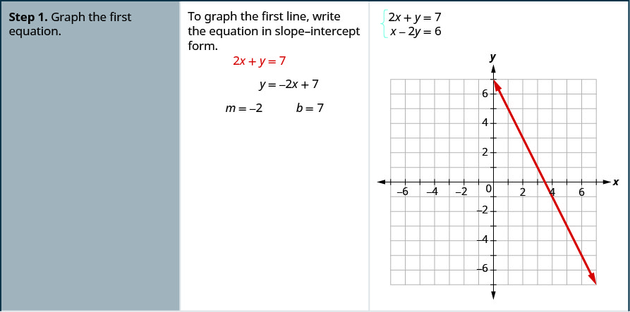
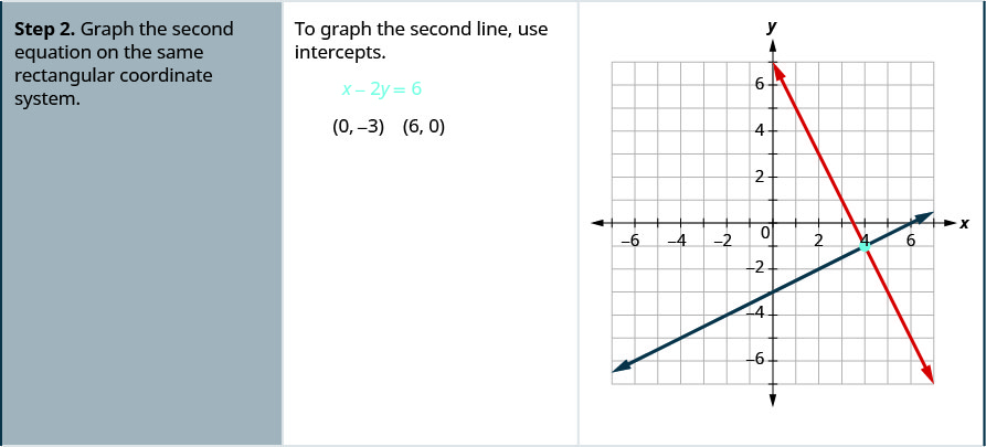
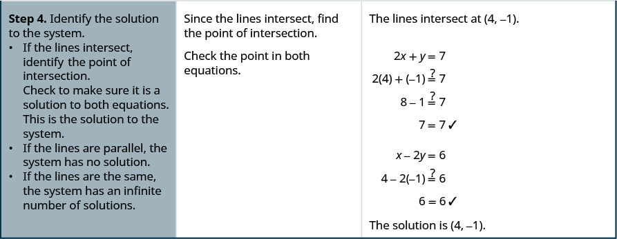
Solve the system by graphing \( \left\{ \begin{array} {l} 2x+y = 7 \\ x−2y = 6 \end{array} \right. \).
- Answer
-

Solve the system by graphing: \( \left\{ \begin{array} {l} x−3y = −3 \\ x+y = 5 \end{array} \right. \).
- Answer
-
\((3,2)\)
Solve the system by graphing: \( \left\{ \begin{array} {l} −x+y = 1 \\ 3x+2y = 12 \end{array} \right.\)
- Answer
-
\((2,3)\)
The steps to use to solve a system of linear equations by graphing are shown here.
- Graph the first equation.
- Graph the second equation on the same rectangular coordinate system.
- Determine whether the lines intersect, are parallel, or are the same line.
- Identify the solution to the system.
- If the lines intersect, identify the point of intersection. This is the solution to the system.
- If the lines are parallel, the system has no solution.
- If the lines are the same, the system has an infinite number of solutions.
- Check the solution in both equations.
In the next example, we’ll first re-write the equations into slope–intercept form as this will make it easy for us to quickly graph the lines.
Solve the system by graphing: \(\left\{ \begin{array} {l} 3x+y = −1 \\ 2x+y = 0 \end{array}\right.\)
- Answer
-
We’ll solve both of these equations for \(y\) so that we can easily graph them using their slopes and \(y\)-intercepts.

Solve the first equation for y. 
Find the slope and y-intercept. 
Solve the second equation for y. 
Find the slope and y-intercept. 
Graph the lines. 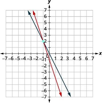
Determine the point of intersection. The lines intersect at \((−1,2)\). Check the solution in both equations.

The solution is \((−1,2)\).
Solve the system by graphing: \(\left\{ \begin{array} {l} −x+y = 1 \\2x+y = 10 \end{array}\right. \).
- Answer
-
\((3,4)\)
Solve the system by graphing: \(\left\{ \begin{array} {l} 2x+y = 6 \\x+y = 1 \end{array}\right. \).
- Answer
-
\((5,−4)\)
In all the systems of linear equations so far, the lines intersected and the solution was one point. In the next two examples, we’ll look at a system of equations that has no solution and at a system of equations that has an infinite number of solutions.
Solve the system by graphing: \(\left\{ \begin{array} {l} y = \tfrac{1}{2}x-3 \\ x-2y = 4 \end{array}\right. \).
- Answer
-

To graph the first equation, we will use its
slope and y-intercept.
To graph the second equation, we will use
the intercepts.

Graph the lines. 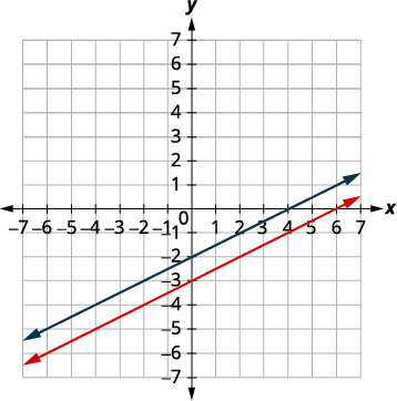
Determine the points of intersection. The lines are parallel.
Since no point is on both lines, there is no
ordered pair that makes both equations
true. There is no solution to this system.
Solve the system by graphing: \(\left\{ \begin{array} {l} y = -\tfrac{1}{4}x+2 \\ x+4y = 4 \end{array}\right. \).
- Answer
-
no solution
Solve the system by graphing: \(\left\{ \begin{array} {l} y = 3x-1 \\ 6x-2y = 6 \end{array}\right. \).
- Answer
-
no solution
Sometimes the equations in a system represent the same line. Since every point on the line makes both equations true, there are infinitely many ordered pairs that make both equations true. There are infinitely many solutions to the system.
Solve the system by graphing: \(\left\{ \begin{array} {l} y = 2x-3 \\ -6x+3y = 9 \end{array}\right. \).
- Answer
-

Find the slope and y-intercept of the first equation. 
Find the intercepts of the second equation. 

Graph the lines. 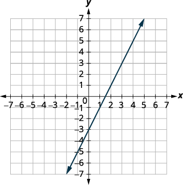
The lines are the same!
Since every point on the line makes both
equations true, there are infinitely many
ordered pairs that make both equations true.
There are infinitely many solutions to this system.If you write the second equation in slope-intercept form, you may recognize that the equations have the same slope and same y-intercept.
Solve the system by graphing: \(\left\{ \begin{array} {l} y = -3x-6 \\ 6x+2y = -12 \end{array}\right. \).
- Answer
-
infinitely many solutions
Solve the system by graphing: \(\left\{ \begin{array} {l} y = \tfrac{1}{2}x-4 \\ 2x-4y = 16 \end{array}\right. \).
- Answer
-
infinitely many solutions
When we graphed the second line in the last example, we drew it right over the first line. We say the two lines are coincident. Coincident lines have the same slope and same y-intercept.
Coincident lines have the same slope and same y-intercept.
The systems of equations in Example and Example each had two intersecting lines. Each system had one solution.
In Example, the equations gave coincident lines, and so the system had infinitely many solutions.
The systems in those three examples had at least one solution. A system of equations that has at least one solution is called a consistent system.
A system with parallel lines, like Example, has no solution. We call a system of equations like this inconsistent. It has no solution.
A consistent system of equations is a system of equations with at least one solution.
An inconsistent system of equations is a system of equations with no solution.
We also categorize the equations in a system of equations by calling the equations independent or dependent. If two equations are independent, they each have their own set of solutions. Intersecting lines and parallel lines are independent.
If two equations are dependent, all the solutions of one equation are also solutions of the other equation. When we graph two dependent equations, we get coincident lines.
Let’s sum this up by looking at the graphs of the three types of systems. See below and Table.
| Lines | Intersecting | Parallel | Coincident |
|---|---|---|---|
| Number of solutions | 1 point | No solution | Infinitely many |
| Consistent/inconsistent | Consistent | Inconsistent | Consistent |
| Dependent/ independent | Independent | Independent | Dependent |
Without graphing, determine the number of solutions and then classify the system of equations.
ⓐ \( \left\{ \begin{array} {l} y = 3x−1 \\ 6x−2y = 12 \end{array}\right. \) ⓑ \( \left\{ \begin{array} {l} 2x+y=−3 \\ x−5y=5 \end{array} \right. \)
- Answer
-
ⓐ We will compare the slopes and intercepts of the two lines.
\(\begin{array} {lll} {} &{} &{ \left\{ \begin{array} {l} {y=3x-1} \\ {6x−2y=12} \end{array} \right. } \\ {} &{} &{y = 3x-1} \\ {\text{The first equation is already in slope-intercept form.}} &{} &{} \\ {\text{Write the second equation in slope-intercept form.}} &{} &{} \\ {} &{} &{} \\ {} &{} &{} \\ {} &{} &{} \\ {} &{} &{6x-2y=12} \\ {} &{} &{-2y=-6x+12} \\ {} &{} &{\frac{-2y}{-2}=\frac{-6x+12}{-2}} \\ {} &{} &{y=3x-6} \\ {} &{y=3x-1} &{y=3x-6} \\ {} &{m=3} &{m=3} \\ {} &{b=-1} &{b=-6} \\ {\text{Find the slope and intercept of each line.}} &{} &{} \\ {} &{} &{} \\ {} &{} &{} \\ {} &{} &{} \\ {} &{} &{} \\ {} &{\text{Since the slopes are the same andy-intercepts are}} &{} \\ {} &{\text{different, the lines are parallel.}} &{} \\ \end{array}\)
ⓑ We will compare the slope and intercepts of the two lines.
\(\begin{array} {lll} {} &{} &{} \\ {} &{ \left\{ \begin{array} {l} 2x+y=-3 \\ x-5y=5 \\ \end{array} \right. } &{} \\ {\text{Write both equations in slope–intercept form.}} &{} &{} \\ {} &{} &{} \\ {} &{} &{} \\ {} &{} &{} \\ {} &{2x+y=-3} &{x-5y=5} \\ {} &{y=-2x-3} &{-5y=-x+5} \\ {} &{} &{\frac{-5y}{-5}=\frac{-x+5}{-5}} \\ {} &{} &{y=\frac{1}{5}-1} \\ {} &{} &{} \\ {} &{} &{} \\ {} &{} &{} \\ {} &{} &{} \\ {\text{Find the slope and intercept of each line.}} &{} &{} \\ {} &{} &{} \\ {} &{y=-2x-3} &{y=\frac{1}{5}-1} \\ {} &{m=-2} &{m=\frac{1}{5}} \\ {} &{b=-3} &{b=-1} \\ {} &{} &{} \\ {} &{\text{Since the slopes are different, the lines intersect.}} &{} \\ \end{array}\)
A system of equations whose graphs are intersect has 1 solution and is consistent and independent.
Without graphing, determine the number of solutions and then classify the system of equations.
ⓐ \(\left\{ \begin{array} {l} y=−2x−4 \\ 4x+2y=9 \end{array} \right. \) ⓑ \(\left\{ \begin{array} {l} 3x+2y=2 \\ 2x+y=1 \end{array} \right. \)
- Answer
-
ⓐ no solution, inconsistent, independent ⓑ one solution, consistent, independent
Without graphing, determine the number of solutions and then classify the system of equations.
ⓐ \(\left\{ \begin{array} {l} y=\frac{1}{3}x−5 \\ x−3y=6 \end{array} \right. \) ⓑ \(\left\{ \begin{array} {l} x+4y=12 \\ −x+y=3 \end{array} \right. \)
- Answer
-
ⓐ no solution, inconsistent, independent ⓑ one solution, consistent, independent
Solving systems of linear equations by graphing is a good way to visualize the types of solutions that may result. However, there are many cases where solving a system by graphing is inconvenient or imprecise. If the graphs extend beyond the small grid with x and y both between \(−10\) and 10, graphing the lines may be cumbersome. And if the solutions to the system are not integers, it can be hard to read their values precisely from a graph.
Solve a System of Equations by Substitution
We will now solve systems of linear equations by the substitution method.
We will use the same system we used first for graphing.
\[ \left\{ \begin{array} {l} 2x+y=7 \\ x−2y=6 \end{array} \right. \nonumber \]
We will first solve one of the equations for either x or y. We can choose either equation and solve for either variable—but we’ll try to make a choice that will keep the work easy.
Then we substitute that expression into the other equation. The result is an equation with just one variable—and we know how to solve those!
After we find the value of one variable, we will substitute that value into one of the original equations and solve for the other variable. Finally, we check our solution and make sure it makes both equations true.
Solve the system by substitution: \( \left\{ \begin{array} {l} 2x+y=7 \\ x−2y=6 \end{array} \right. \)
- Answer
-


Solve the system by substitution: \( \left\{ \begin{array} {l} −2x+y=−11 \\ x+3y=9 \end{array} \right. \)
- Answer
-
\((6,1)\)
Solve the system by substitution: \( \left\{ \begin{array} {l} 2x+y=−1 \\ 4x+3y=3 \end{array} \right. \)
- Answer
-
\((−3,5)\)
- Solve one of the equations for either variable.
- Substitute the expression from Step 1 into the other equation.
- Solve the resulting equation.
- Substitute the solution in Step 3 into either of the original equations to find the other variable.
- Write the solution as an ordered pair.
- Check that the ordered pair is a solution to both original equations.
Be very careful with the signs in the next example.
Solve the system by substitution: \( \left\{ \begin{array} {l} 4x+2y=4 \\ 6x−y=8 \end{array} \right. \)
- Answer
-
We need to solve one equation for one variable. We will solve the first equation for y.

Solve the first equation for y.
Substitute \(−2x+2\) for y in the second equation.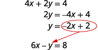
Replace the y with \(−2x+2\). 
Solve the equation for x. 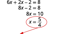
Substitute \(x=54\) into \(4x+2y=4\) to find y. 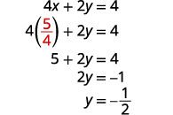
The ordered pair is \((54,−12)\). Check the ordered pair in both equations.
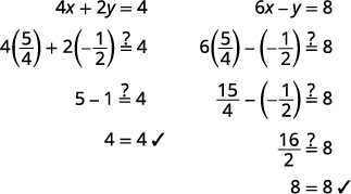
The solution is \((54,−12)\).
Solve the system by substitution: \( \left\{ \begin{array} {l} x−4y=−4 \\ −3x+4y=0 \end{array} \right. \)
- Answer
-
\((2,32)\)
Solve the system by substitution: \( \left\{ \begin{array} {l} 4x−y=0 \\ 2x−3y=5 \end{array} \right. \)
- Answer
-
\((−12,−2)\)
Solve a System of Equations by Elimination
We have solved systems of linear equations by graphing and by substitution. Graphing works well when the variable coefficients are small and the solution has integer values. Substitution works well when we can easily solve one equation for one of the variables and not have too many fractions in the resulting expression.
The third method of solving systems of linear equations is called the Elimination Method. When we solved a system by substitution, we started with two equations and two variables and reduced it to one equation with one variable. This is what we’ll do with the elimination method, too, but we’ll have a different way to get there.
The Elimination Method is based on the Addition Property of Equality. The Addition Property of Equality says that when you add the same quantity to both sides of an equation, you still have equality. We will extend the Addition Property of Equality to say that when you add equal quantities to both sides of an equation, the results are equal.
For any expressions a, b, c, and d.
\[\begin{array} {ll} {\text{if}} &{a=b} \\ {\text{and}} &{c=d} \\ {\text{then}} &{a+c=b+d.} \\ \nonumber \end{array}\]
To solve a system of equations by elimination, we start with both equations in standard form. Then we decide which variable will be easiest to eliminate. How do we decide? We want to have the coefficients of one variable be opposites, so that we can add the equations together and eliminate that variable.
Notice how that works when we add these two equations together:
\[\left\{ \begin{array} {l} 3x+y=5 \\ \underline{2x−y=0} \end{array} \right. \nonumber\]
\[5x=5 \nonumber\]
The y’s add to zero and we have one equation with one variable.
Let’s try another one:
\[ \left\{ \begin{array} x+4y=2 \\ 2x+5y=−2 \end{array} \right. \nonumber\]
This time we don’t see a variable that can be immediately eliminated if we add the equations.
But if we multiply the first equation by \(−2\), we will make the coefficients of x opposites. We must multiply every term on both sides of the equation by \(−2\).

Then rewrite the system of equations.

Now we see that the coefficients of the x terms are opposites, so x will be eliminated when we add these two equations.

Once we get an equation with just one variable, we solve it. Then we substitute that value into one of the original equations to solve for the remaining variable. And, as always, we check our answer to make sure it is a solution to both of the original equations.
Now we’ll see how to use elimination to solve the same system of equations we solved by graphing and by substitution.
Solve the system by elimination: \(\left\{ \begin{array} {l} 2x+y=7 \\ x−2y=6 \end{array} \right. \)
- Answer
-


Solve the system by elimination: \(\left\{ \begin{array} {l} 3x+y=5 \\ 2x−3y=7 \end{array} \right.\)
- Answer
-
\((2,−1)\)
Solve the system by elimination: \(\left\{ \begin{array} {l} 4x+y=−5 \\ −2x−2y=−2 \end{array} \right.\)
- Answer
-
\((−2,3)\)
The steps are listed here for easy reference.
- Write both equations in standard form. If any coefficients are fractions, clear them.
- Make the coefficients of one variable opposites.
- Decide which variable you will eliminate.
- Multiply one or both equations so that the coefficients of that variable are opposites.
- Add the equations resulting from Step 2 to eliminate one variable.
- Solve for the remaining variable.
- Substitute the solution from Step 4 into one of the original equations. Then solve for the other variable.
- Write the solution as an ordered pair.
- Check that the ordered pair is a solution to both original equations.
Now we’ll do an example where we need to multiply both equations by constants in order to make the coefficients of one variable opposites.
Solve the system by elimination: \(\left\{ \begin{array} {l} 4x−3y=9 \\ 7x+2y=−6 \end{array} \right. \)
- Answer
-
In this example, we cannot multiply just one equation by any constant to get opposite coefficients. So we will strategically multiply both equations by different constants to get the opposites.

Both equations are in standard form.
To get opposite coefficients of y, we will
multiply the first equation by 2 and the
second equation by 3.
Simplify. 
Add the two equations to eliminate y. 
Solve for x. 
Substitute x=0x=0 into one of the original equations. 
Solve for y. 
Write the solution as an ordered pair. The ordered pair is \((0,−3)\).
Check that the ordered pair is a solution to
both original equations.

The solution is \((0,−3)\).
Solve the system by elimination: \(\left\{ \begin{array} {l} 3x−4y=−9 \\ 5x+3y=14\end{array} \right. \)
- Answer
-
\((1,3)\)
Solve each system by elimination: \(\left\{ \begin{array} {l} 7x+8y=4 \\ 3x−5y=27 \end{array} \right.\)
- Answer
-
\((4,−3)\)
When the system of equations contains fractions, we will first clear the fractions by multiplying each equation by the LCD of all the fractions in the equation.
Solve the system by elimination: \(\left\{ \begin{array} {l} x+\tfrac{1}{2}y=6 \\ \tfrac{3}{2}x+\tfrac{2}{3}y=\tfrac{17}{2} \end{array} \right.\)
- Answer
-
In this example, both equations have fractions. Our first step will be to multiply each equation by the LCD of all the fractions in the equation to clear the fractions.

To clear the fractions, multiply each
equation by its LCD.
Simplify. 
Now we are ready to eliminate one
of the variables. Notice that both equations are in
standard form.We can eliminate y by multiplying the top equation by \(−4\). 
Simplify and add.
Substitute \(x=3\) into one of the original equations.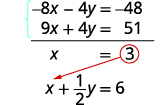
Solve for y. 


Write the solution as an ordered pair. The ordered pair is \((3,6)\). Check that the ordered pair is a solution to
both original equations.
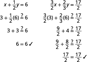
The solution is \((3,6)\).
Solve each system by elimination: \(\left\{ \begin{array} {l} \tfrac{1}{3}x−\tfrac{1}{2}y=1 \\ \tfrac{3}{4}x−y=\tfrac{5}{2} \end{array} \right.\)
- Answer
-
\((6,2)\)
Solve each system by elimination: \(\left\{ \begin{array} {l} x+\tfrac{3}{5}y=−\tfrac{1}{5} \\ −\tfrac{1}{2}x−\tfrac{2}{3}y=\tfrac{5}{6} \end{array} \right.\)
- Answer
-
\((1,−2)\)
When we solved the system by graphing, we saw that not all systems of linear equations have a single ordered pair as a solution. When the two equations were really the same line, there were infinitely many solutions. We called that a consistent system. When the two equations described parallel lines, there was no solution. We called that an inconsistent system.
The same is true using substitution or elimination. If the equation at the end of substitution or elimination is a true statement, we have a consistent but dependent system and the system of equations has infinitely many solutions. If the equation at the end of substitution or elimination is a false statement, we have an inconsistent system and the system of equations has no solution.
Solve the system by elimination: \(\left\{ \begin{array} {l} 3x+4y=12 \\ y=3−\tfrac{3}{4}x \end{array} \right. \)
- Answer
-
\(\begin{array} {ll} {} &{ \left\{ \begin{array} {l} 3x+4y=12 \\ y=3−\frac{3}{4}x \end{array} \right.} \\ {} &{} \\ {\text{Write the second equation in standard form.}} &{\left\{ \begin{array} {l} 3x+4y=12 \\ \frac{3}{4}x+y=3 \end{array} \right. } \\ {} &{} \\ {\text{Clear the fractions by multiplying the } \\ \text{second equation by 4.}} &{\left\{ \begin{array} {l} 3x+4y=12 \\ 4(\frac{3}{4}x+y)=4(3) \end{array} \right. } \\ {} &{} \\ {\text{Simplify.}} &{\left\{ \begin{array} {l} 3x+4y=12 \\ 3x+4y=12 \end{array} \right. } \\ {} &{} \\ {\text{To eliminate a variable, we multiply the} \\ \text{second equation by−1. Simplify and add.}} &{\begin{array} {l} {\left\{ \begin{array} {l} 3x+4y=12 \\ \underline{-3x-4y=-12 } \end{array} \right.} \\ {\hspace{16mm} 0=0} \end{array}} \\ \end{array} \)
This is a true statement. The equations are consistent but dependent. Their graphs would be the same line. The system has infinitely many solutions.
After we cleared the fractions in the second equation, did you notice that the two equations were the same? That means we have coincident lines.
Solve the system by elimination: \(\left\{ \begin{array} {l} 5x−3y=15 \\ 5y=−5+\tfrac{5}{3}x \end{array} \right. \)
- Answer
-
infinitely many solutions
Solve the system by elimination: \(\left\{ \begin{array} {l} x+2y=6 \\ y=−\tfrac{1}{2}x+3\end{array} \right. \)
- Answer
-
infinitely many solutions
Choose the Most Convenient Method to Solve a System of Linear Equations
When you solve a system of linear equations in in an application, you will not be told which method to use. You will need to make that decision yourself. So you’ll want to choose the method that is easiest to do and minimizes your chance of making mistakes.
\[ \textbf{Choose the Most Convenient Method to Solve a System of Linear Equations} \\ \begin{array} {lll} {\underline{\textbf{Graphing}}} &{\underline{\textbf{Substitution}}} &{\underline{\textbf{Elimination}}} \\ {\text{Use when you need a}} &{\text{Use when one equation is}} &{\text{Use when the equations a}} \\ {\text{picture of the situation.}} &{\text{already solved or can be}} &{\text{rein standard form.}} \\ {\text{}} &{\text{easily solved for one}} &{\text{}} \\ {\text{}} &{\text{variable.}} &{\text{}} \\ \end{array} \nonumber \]
For each system of linear equations, decide whether it would be more convenient to solve it by substitution or elimination. Explain your answer.
ⓐ \(\left\{ \begin{array} {l} 3x+8y=40 \\ 7x−4y=−32 \end{array} \right.\) ⓑ \(\left\{ \begin{array} {l} 5x+6y=12 \\ y=\tfrac{2}{3}x−1 \end{array} \right.\)
- Answer
-
ⓐ
\[\left\{ \begin{array} {l} 3x+8y=40 \\ 7x−4y=−32 \end{array} \right.\nonumber\]
Since both equations are in standard form, using elimination will be most convenient.
ⓑ
\[\left\{ \begin{array} {l} 5x+6y=12 \\ y=\tfrac{2}{3}x−1 \end{array} \right.\nonumber \]
Since one equation is already solved for y, using substitution will be most convenient.
For each system of linear equations decide whether it would be more convenient to solve it by substitution or elimination. Explain your answer.
ⓐ \(\left\{ \begin{array} {l} 4x−5y=−32 \\ 3x+2y=−1 \end{array} \right.\) ⓑ \(\left\{ \begin{array} {l} x=2y−1 \\ 3x−5y=−7 \end{array} \right.\)
- Answer
-
ⓐ Since both equations are in standard form, using elimination will be most convenient. ⓑ Since one equation is already solved for x, using substitution will be most convenient.
For each system of linear equations decide whether it would be more convenient to solve it by substitution or elimination. Explain your answer.
ⓐ \(\left\{ \begin{array} {l} y=2x−1 \\ 3x−4y=−6 \end{array} \right.\) ⓑ \(\left\{ \begin{array} {l} 6x−2y=12 \\ 3x+7y=−13 \end{array} \right.\)
- Answer
-
ⓐ Since one equation is already solved for y, using substitution will be most convenient. ⓑ Since both equations are in standard form, using elimination will be most convenient.
Key Concepts
- How to solve a system of linear equations by graphing.
- Graph the first equation.
- Graph the second equation on the same rectangular coordinate system.
- Determine whether the lines intersect, are parallel, or are the same line.
- Identify the solution to the system.
If the lines intersect, identify the point of intersection. This is the solution to the system.
If the lines are parallel, the system has no solution.
If the lines are the same, the system has an infinite number of solutions. - Check the solution in both equations.
- How to solve a system of equations by substitution.
- Solve one of the equations for either variable.
- Substitute the expression from Step 1 into the other equation.
- Solve the resulting equation.
- Substitute the solution in Step 3 into either of the original equations to find the other variable.
- Write the solution as an ordered pair.
- Check that the ordered pair is a solution to both original equations.
- How to solve a system of equations by elimination.
- Write both equations in standard form. If any coefficients are fractions, clear them.
- Make the coefficients of one variable opposites.
Decide which variable you will eliminate.
Multiply one or both equations so that the coefficients of that variable are opposites. - Add the equations resulting from Step 2 to eliminate one variable.
- Solve for the remaining variable.
- Substitute the solution from Step 4 into one of the original equations. Then solve for the other variable.
- Write the solution as an ordered pair.
- Check that the ordered pair is a solution to both original equations. \[ \textbf{Choose the Most Convenient Method to Solve a System of Linear Equations} \\ \begin{array} {lll} {\underline{\textbf{Graphing}}} &{\underline{\textbf{Substitution}}} &{\underline{\textbf{Elimination}}} \\ {\text{}} &{\text{Use when one equation is}} &{\text{}} \\ {\text{Use when you need a}} &{\text{already solved or can be}} &{\text{Use when the equations a}} \\ {\text{picture of the situation.}} &{\text{easily solved for one}} &{\text{rein standard form.}} \\ {\text{}} &{\text{variable.}} &{\text{}} \\ \end{array} \nonumber \]
Glossary
- coincident lines
- Coincident lines have the same slope and same y-intercept.
- consistent and inconsistent systems
- Consistent system of equations is a system of equations with at least one solution; inconsistent system of equations is a system of equations with no solution.
- solutions of a system of equations
- Solutions of a system of equations are the values of the variables that make all the equations true; solution is represented by an ordered pair (x,y).(x,y).
- system of linear equations
- When two or more linear equations are grouped together, they form a system of linear equations.


