
13.1: Introduction to Conics
- Page ID
- 45123

\( \newcommand{\vecs}[1]{\overset { \scriptstyle \rightharpoonup} {\mathbf{#1}} } \)
\( \newcommand{\vecd}[1]{\overset{-\!-\!\rightharpoonup}{\vphantom{a}\smash {#1}}} \)
\( \newcommand{\id}{\mathrm{id}}\) \( \newcommand{\Span}{\mathrm{span}}\)
( \newcommand{\kernel}{\mathrm{null}\,}\) \( \newcommand{\range}{\mathrm{range}\,}\)
\( \newcommand{\RealPart}{\mathrm{Re}}\) \( \newcommand{\ImaginaryPart}{\mathrm{Im}}\)
\( \newcommand{\Argument}{\mathrm{Arg}}\) \( \newcommand{\norm}[1]{\| #1 \|}\)
\( \newcommand{\inner}[2]{\langle #1, #2 \rangle}\)
\( \newcommand{\Span}{\mathrm{span}}\)
\( \newcommand{\id}{\mathrm{id}}\)
\( \newcommand{\Span}{\mathrm{span}}\)
\( \newcommand{\kernel}{\mathrm{null}\,}\)
\( \newcommand{\range}{\mathrm{range}\,}\)
\( \newcommand{\RealPart}{\mathrm{Re}}\)
\( \newcommand{\ImaginaryPart}{\mathrm{Im}}\)
\( \newcommand{\Argument}{\mathrm{Arg}}\)
\( \newcommand{\norm}[1]{\| #1 \|}\)
\( \newcommand{\inner}[2]{\langle #1, #2 \rangle}\)
\( \newcommand{\Span}{\mathrm{span}}\) \( \newcommand{\AA}{\unicode[.8,0]{x212B}}\)
\( \newcommand{\vectorA}[1]{\vec{#1}} % arrow\)
\( \newcommand{\vectorAt}[1]{\vec{\text{#1}}} % arrow\)
\( \newcommand{\vectorB}[1]{\overset { \scriptstyle \rightharpoonup} {\mathbf{#1}} } \)
\( \newcommand{\vectorC}[1]{\textbf{#1}} \)
\( \newcommand{\vectorD}[1]{\overrightarrow{#1}} \)
\( \newcommand{\vectorDt}[1]{\overrightarrow{\text{#1}}} \)
\( \newcommand{\vectE}[1]{\overset{-\!-\!\rightharpoonup}{\vphantom{a}\smash{\mathbf {#1}}}} \)
\( \newcommand{\vecs}[1]{\overset { \scriptstyle \rightharpoonup} {\mathbf{#1}} } \)
\( \newcommand{\vecd}[1]{\overset{-\!-\!\rightharpoonup}{\vphantom{a}\smash {#1}}} \)
\(\newcommand{\avec}{\mathbf a}\) \(\newcommand{\bvec}{\mathbf b}\) \(\newcommand{\cvec}{\mathbf c}\) \(\newcommand{\dvec}{\mathbf d}\) \(\newcommand{\dtil}{\widetilde{\mathbf d}}\) \(\newcommand{\evec}{\mathbf e}\) \(\newcommand{\fvec}{\mathbf f}\) \(\newcommand{\nvec}{\mathbf n}\) \(\newcommand{\pvec}{\mathbf p}\) \(\newcommand{\qvec}{\mathbf q}\) \(\newcommand{\svec}{\mathbf s}\) \(\newcommand{\tvec}{\mathbf t}\) \(\newcommand{\uvec}{\mathbf u}\) \(\newcommand{\vvec}{\mathbf v}\) \(\newcommand{\wvec}{\mathbf w}\) \(\newcommand{\xvec}{\mathbf x}\) \(\newcommand{\yvec}{\mathbf y}\) \(\newcommand{\zvec}{\mathbf z}\) \(\newcommand{\rvec}{\mathbf r}\) \(\newcommand{\mvec}{\mathbf m}\) \(\newcommand{\zerovec}{\mathbf 0}\) \(\newcommand{\onevec}{\mathbf 1}\) \(\newcommand{\real}{\mathbb R}\) \(\newcommand{\twovec}[2]{\left[\begin{array}{r}#1 \\ #2 \end{array}\right]}\) \(\newcommand{\ctwovec}[2]{\left[\begin{array}{c}#1 \\ #2 \end{array}\right]}\) \(\newcommand{\threevec}[3]{\left[\begin{array}{r}#1 \\ #2 \\ #3 \end{array}\right]}\) \(\newcommand{\cthreevec}[3]{\left[\begin{array}{c}#1 \\ #2 \\ #3 \end{array}\right]}\) \(\newcommand{\fourvec}[4]{\left[\begin{array}{r}#1 \\ #2 \\ #3 \\ #4 \end{array}\right]}\) \(\newcommand{\cfourvec}[4]{\left[\begin{array}{c}#1 \\ #2 \\ #3 \\ #4 \end{array}\right]}\) \(\newcommand{\fivevec}[5]{\left[\begin{array}{r}#1 \\ #2 \\ #3 \\ #4 \\ #5 \\ \end{array}\right]}\) \(\newcommand{\cfivevec}[5]{\left[\begin{array}{c}#1 \\ #2 \\ #3 \\ #4 \\ #5 \\ \end{array}\right]}\) \(\newcommand{\mattwo}[4]{\left[\begin{array}{rr}#1 \amp #2 \\ #3 \amp #4 \\ \end{array}\right]}\) \(\newcommand{\laspan}[1]{\text{Span}\{#1\}}\) \(\newcommand{\bcal}{\cal B}\) \(\newcommand{\ccal}{\cal C}\) \(\newcommand{\scal}{\cal S}\) \(\newcommand{\wcal}{\cal W}\) \(\newcommand{\ecal}{\cal E}\) \(\newcommand{\coords}[2]{\left\{#1\right\}_{#2}}\) \(\newcommand{\gray}[1]{\color{gray}{#1}}\) \(\newcommand{\lgray}[1]{\color{lightgray}{#1}}\) \(\newcommand{\rank}{\operatorname{rank}}\) \(\newcommand{\row}{\text{Row}}\) \(\newcommand{\col}{\text{Col}}\) \(\renewcommand{\row}{\text{Row}}\) \(\newcommand{\nul}{\text{Nul}}\) \(\newcommand{\var}{\text{Var}}\) \(\newcommand{\corr}{\text{corr}}\) \(\newcommand{\len}[1]{\left|#1\right|}\) \(\newcommand{\bbar}{\overline{\bvec}}\) \(\newcommand{\bhat}{\widehat{\bvec}}\) \(\newcommand{\bperp}{\bvec^\perp}\) \(\newcommand{\xhat}{\widehat{\xvec}}\) \(\newcommand{\vhat}{\widehat{\vvec}}\) \(\newcommand{\uhat}{\widehat{\uvec}}\) \(\newcommand{\what}{\widehat{\wvec}}\) \(\newcommand{\Sighat}{\widehat{\Sigma}}\) \(\newcommand{\lt}{<}\) \(\newcommand{\gt}{>}\) \(\newcommand{\amp}{&}\) \(\definecolor{fillinmathshade}{gray}{0.9}\)Recall, a line segment is a line with two points on each end:

Let’s take this line segment and place it on the Cartesian coordinate plane:

We can see that once we place the line segment on the Cartesian coordinate plane, points \(A\) and \(B\) will have \(x\) and \(y\) coordinates. Let’s see the coordinates instead of \(A\) and \(B\):
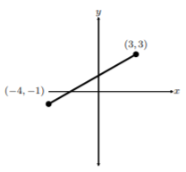
Since the line segment has endpoints in which are ordered pairs, we can find the distance of this line segment. In fact, if we used the Pythagorean Theorem to find this length, we would obtain length \(\sqrt{65}\):
Pythagorean Theorem: \(a^2+b^2=c^2\)
\[\begin{aligned}a^2+b^2&=c^2 \\ 7^2+4^2&=c^2 \\ 49+16&=c^2 \\ 65&=c^2 \\ \sqrt{65}&=c\end{aligned}\]

The next step is to find a more sophisticated way to find the distance between any two points no matter the location. Take moment to think about it. If the two points are at \((−100, 2000)\) and \((300, 5000)\), are we going to draw a right triangle that large to apply the Pythagorean Theorem? No way! Let’s work smarter and not harder. Let’s place two generic points where we had \((−4, −1)\) and \((3, 3)\) and apply the Pythagorean Theorem to find the hypotenuse:
Pythagorean Theorem: \(a^2+b^2=c^2\)
\[\begin{aligned}a^2+b^2&=c^2 \\ (x_2-x_1)^2 +(y_2-y_1)^2 &=c^2 \\ \sqrt{(x_2-x_1)^2+(y_2-y_1)^2}&=c\end{aligned}\]

Thus, we have found a generic formula to obtain the distance between any two points on the Cartesian coordinate plane.
The Distance Formula
Given two points, \((x_1, y_1)\) and \((x_2, y_2)\) on a line segment, the distance, \(d\), from \((x_1, y_1)\) to \((x_2, y_2)\) is given by
\[d=\sqrt{(x_2-x_1)^2+(y_2-y_1)^2}\nonumber\]
Find the distance between the points \((−2, 1)\) and \((1, 2)\). Leave your answer in exact form, i.e., your answer should contain a square root.
Solution
To find the distance between the points \((−2, 1)\) and \((1, 2)\), we can apply the distance formula:
\[\begin{aligned}d&=\sqrt{(1-(-2))^2+(2-1)^2} \\ &=\sqrt{(3)^2+(1)^2} \\ &=\sqrt{9+1} \\ &=\sqrt{10}\end{aligned}\]
Since the directions insisted we leave the answer in exact form, then we leave \(d=\sqrt{10}\).
In the study of Euclidean geometry, we call this (most common) type of distance Euclidean distance, as it is derived from the Pythagorean theorem, which does not hold in non-Euclidean geometries. The Euclidean distance between two objects may also be generalized to the case where the objects are no longer points but are higher-dimensional manifolds, such as space curves.
The Midpoint Formula
If we can calculate the distance between two points, then we certainly should be able to find the midpoint between two points. In fact, all we do is calculate the average between the corresponding coordinates, i.e., the \(x\) coordinate of the midpoint is the average of the two given \(x\) coordinates in the ordered pairs \((x_1, y_1)\) and \((x_2, y_2)\):
\[x_m=\dfrac{x_1+x_2}{2}\nonumber\]
Similarly, for the \(y\) coordinate of the midpoint, it is the average of the two given \(y\) coordinates in the ordered pairs \((x_1, y_1)\) and \((x_2, y_2)\):
\[y_m=\dfrac{y_1+y_2}{2}\nonumber\]
Given two points, \((x_1, y_1)\) and \((x_2, y_2)\) on a line segment, the midpoint, \(m\), from \((x_1, y_1)\) to \((x_2, y_2)\) is given by
\[(x_m,y_m)=\left(\dfrac{x_2+x_1}{2},\dfrac{y_2+y_1}{2}\right)\nonumber\]

Find the midpoint of the line segment from \((−4, 2)\) to \((2, −3)\).
Solution
To find the midpoint between the points \((−4, 2)\) and \((2, −3)\), we can apply the midpoint formula for each coordinate:
\[\begin{aligned} (x_m,y_m)&=\left(\dfrac{x_2+x_1}{2},\dfrac{y_2+y_1}{2}\right) \\ &=\left(\dfrac{2+(-4)}{2},\dfrac{(-3)+2}{2}\right) \\ &=\left(\dfrac{-2}{2},\dfrac{-1}{2}\right) \\ &=\left(-1,-\dfrac{1}{2}\right)\end{aligned}\]
Thus, the midpoint between \((−4, 2)\) to \((2, −3)\) is \(\left(-1,-\dfrac{1}{2}\right)\).
Constructing a Conic
To understand the idea of conics, we begin with a shape that is familiar to all of us, a right circular cone. Let’s look at a right circular cone:

Next, we can take a plane and cut through the cone so that the plane is parallel to the cone’s base:
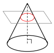
When we took the plane and cut the cone so that the plane is parallel to the cone’s base, notice we made a familiar shape- the circle. Wow! So cool, right? Let’s try another one. Let’s take the plane and cut the cone so that the plane is parallel to the cone:
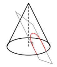
When we took the plane and cut the cone so that the plane is parallel to the cone, notice we made another familiar shape. In fact, we know this conic very well from a previous chapter- the parabola. Amazing! All we did was take a right circular cone, cut through it with a plane, and then obtained two very well-known conics.
If we take a right circular cone and cut the cone so that the plane is parallel to
- the cone’s base, then we obtain a circle.
- the opposite side of the cone, then we obtain a parabola.


There are two more conics, the ellipse and hyperbola, which are two other type of cuts from the cone. However, we only discuss the circle and parabola in this textbook. The ellipse and hyperbola are discussed in a future mathematics course.


Introduction to Conics Homework
Find the midpoint and distance between the given two points.
From \((−5, −1)\) to \((5, 2)\)
From \((4, −4)\) to \((2, 5)\)
From \((1, 1)\) to \((−2, −4)\)
From \((5, −2)\) to \((−5, −5)\)
From \((88, −89)\) to \((97, −49)\)
From \((−77, 21)\) to \((−42, 9)\)
Identify each conic by its graph or equation.
\(y-1=(x-3)^2\)
\(x^2+y^2=25\)
\(y-4=(x-3)^2\)
\(x^2+y^2=16\)