1.2: Graphs and Symmetry
- Page ID
- 226
\( \newcommand{\vecs}[1]{\overset { \scriptstyle \rightharpoonup} {\mathbf{#1}} } \)
\( \newcommand{\vecd}[1]{\overset{-\!-\!\rightharpoonup}{\vphantom{a}\smash {#1}}} \)
\( \newcommand{\dsum}{\displaystyle\sum\limits} \)
\( \newcommand{\dint}{\displaystyle\int\limits} \)
\( \newcommand{\dlim}{\displaystyle\lim\limits} \)
\( \newcommand{\id}{\mathrm{id}}\) \( \newcommand{\Span}{\mathrm{span}}\)
( \newcommand{\kernel}{\mathrm{null}\,}\) \( \newcommand{\range}{\mathrm{range}\,}\)
\( \newcommand{\RealPart}{\mathrm{Re}}\) \( \newcommand{\ImaginaryPart}{\mathrm{Im}}\)
\( \newcommand{\Argument}{\mathrm{Arg}}\) \( \newcommand{\norm}[1]{\| #1 \|}\)
\( \newcommand{\inner}[2]{\langle #1, #2 \rangle}\)
\( \newcommand{\Span}{\mathrm{span}}\)
\( \newcommand{\id}{\mathrm{id}}\)
\( \newcommand{\Span}{\mathrm{span}}\)
\( \newcommand{\kernel}{\mathrm{null}\,}\)
\( \newcommand{\range}{\mathrm{range}\,}\)
\( \newcommand{\RealPart}{\mathrm{Re}}\)
\( \newcommand{\ImaginaryPart}{\mathrm{Im}}\)
\( \newcommand{\Argument}{\mathrm{Arg}}\)
\( \newcommand{\norm}[1]{\| #1 \|}\)
\( \newcommand{\inner}[2]{\langle #1, #2 \rangle}\)
\( \newcommand{\Span}{\mathrm{span}}\) \( \newcommand{\AA}{\unicode[.8,0]{x212B}}\)
\( \newcommand{\vectorA}[1]{\vec{#1}} % arrow\)
\( \newcommand{\vectorAt}[1]{\vec{\text{#1}}} % arrow\)
\( \newcommand{\vectorB}[1]{\overset { \scriptstyle \rightharpoonup} {\mathbf{#1}} } \)
\( \newcommand{\vectorC}[1]{\textbf{#1}} \)
\( \newcommand{\vectorD}[1]{\overrightarrow{#1}} \)
\( \newcommand{\vectorDt}[1]{\overrightarrow{\text{#1}}} \)
\( \newcommand{\vectE}[1]{\overset{-\!-\!\rightharpoonup}{\vphantom{a}\smash{\mathbf {#1}}}} \)
\( \newcommand{\vecs}[1]{\overset { \scriptstyle \rightharpoonup} {\mathbf{#1}} } \)
\(\newcommand{\longvect}{\overrightarrow}\)
\( \newcommand{\vecd}[1]{\overset{-\!-\!\rightharpoonup}{\vphantom{a}\smash {#1}}} \)
\(\newcommand{\avec}{\mathbf a}\) \(\newcommand{\bvec}{\mathbf b}\) \(\newcommand{\cvec}{\mathbf c}\) \(\newcommand{\dvec}{\mathbf d}\) \(\newcommand{\dtil}{\widetilde{\mathbf d}}\) \(\newcommand{\evec}{\mathbf e}\) \(\newcommand{\fvec}{\mathbf f}\) \(\newcommand{\nvec}{\mathbf n}\) \(\newcommand{\pvec}{\mathbf p}\) \(\newcommand{\qvec}{\mathbf q}\) \(\newcommand{\svec}{\mathbf s}\) \(\newcommand{\tvec}{\mathbf t}\) \(\newcommand{\uvec}{\mathbf u}\) \(\newcommand{\vvec}{\mathbf v}\) \(\newcommand{\wvec}{\mathbf w}\) \(\newcommand{\xvec}{\mathbf x}\) \(\newcommand{\yvec}{\mathbf y}\) \(\newcommand{\zvec}{\mathbf z}\) \(\newcommand{\rvec}{\mathbf r}\) \(\newcommand{\mvec}{\mathbf m}\) \(\newcommand{\zerovec}{\mathbf 0}\) \(\newcommand{\onevec}{\mathbf 1}\) \(\newcommand{\real}{\mathbb R}\) \(\newcommand{\twovec}[2]{\left[\begin{array}{r}#1 \\ #2 \end{array}\right]}\) \(\newcommand{\ctwovec}[2]{\left[\begin{array}{c}#1 \\ #2 \end{array}\right]}\) \(\newcommand{\threevec}[3]{\left[\begin{array}{r}#1 \\ #2 \\ #3 \end{array}\right]}\) \(\newcommand{\cthreevec}[3]{\left[\begin{array}{c}#1 \\ #2 \\ #3 \end{array}\right]}\) \(\newcommand{\fourvec}[4]{\left[\begin{array}{r}#1 \\ #2 \\ #3 \\ #4 \end{array}\right]}\) \(\newcommand{\cfourvec}[4]{\left[\begin{array}{c}#1 \\ #2 \\ #3 \\ #4 \end{array}\right]}\) \(\newcommand{\fivevec}[5]{\left[\begin{array}{r}#1 \\ #2 \\ #3 \\ #4 \\ #5 \\ \end{array}\right]}\) \(\newcommand{\cfivevec}[5]{\left[\begin{array}{c}#1 \\ #2 \\ #3 \\ #4 \\ #5 \\ \end{array}\right]}\) \(\newcommand{\mattwo}[4]{\left[\begin{array}{rr}#1 \amp #2 \\ #3 \amp #4 \\ \end{array}\right]}\) \(\newcommand{\laspan}[1]{\text{Span}\{#1\}}\) \(\newcommand{\bcal}{\cal B}\) \(\newcommand{\ccal}{\cal C}\) \(\newcommand{\scal}{\cal S}\) \(\newcommand{\wcal}{\cal W}\) \(\newcommand{\ecal}{\cal E}\) \(\newcommand{\coords}[2]{\left\{#1\right\}_{#2}}\) \(\newcommand{\gray}[1]{\color{gray}{#1}}\) \(\newcommand{\lgray}[1]{\color{lightgray}{#1}}\) \(\newcommand{\rank}{\operatorname{rank}}\) \(\newcommand{\row}{\text{Row}}\) \(\newcommand{\col}{\text{Col}}\) \(\renewcommand{\row}{\text{Row}}\) \(\newcommand{\nul}{\text{Nul}}\) \(\newcommand{\var}{\text{Var}}\) \(\newcommand{\corr}{\text{corr}}\) \(\newcommand{\len}[1]{\left|#1\right|}\) \(\newcommand{\bbar}{\overline{\bvec}}\) \(\newcommand{\bhat}{\widehat{\bvec}}\) \(\newcommand{\bperp}{\bvec^\perp}\) \(\newcommand{\xhat}{\widehat{\xvec}}\) \(\newcommand{\vhat}{\widehat{\vvec}}\) \(\newcommand{\uhat}{\widehat{\uvec}}\) \(\newcommand{\what}{\widehat{\wvec}}\) \(\newcommand{\Sighat}{\widehat{\Sigma}}\) \(\newcommand{\lt}{<}\) \(\newcommand{\gt}{>}\) \(\newcommand{\amp}{&}\) \(\definecolor{fillinmathshade}{gray}{0.9}\)Symmetry (Geometry)
Definition: Symmetric with respect to the y-axis
We say that a graph is symmetric with respect to the y-axis if for every point \((a,b)\) on the graph, there is also a point \((-a,b)\) on the graph; hence \[f(x,y) = f(-x,y).\]
Visually we have that the y-axis acts as a mirror for the graph. We will demonstrate several functions to test for symmetry graphically using the graphing calculator.

Definition: Symmetric with respect to the x-axis
We say that a graph is symmetric with respect to the x axis if for every point \((a,b)\) on the graph, there is also a point \((a,-b)\) on the graph; hence \[f(x,y) = f(x,-y).\]
Visually we have that the x-axis acts as a mirror for the graph. We will demonstrate several functions to test for symmetry graphically using the graphing calculator.
Definition: Symmetry with respect to Origin
We say that a graph is symmetric with respect to the origin if for every point \((a,b)\) on the graph, there is also a point \((-a,-b)\) on the graph; hence \[f(x,y) = f(-x,-y).\]
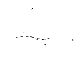
Visually we have that given a point \(P\) on the graph if we draw a line segment \(PQ\) through \(P\) and the origin such that the origin is the midpoint of \(PQ\), then \(Q\) is also on the graph.

We will use the graphing calculator to test for all three symmetries.
Symmetry (Algebra)
x-axis Symmetry
To test algebraically if a graph is symmetric with respect the x-axis, we replace all the \(y\)'s with \(-y\) and see if we get an equivalent expression.
Example \(\PageIndex{1}\)
For
\[x - 2y = 5 \]
we replace with
\[ x - 2(-y) = 5.\]
Simplifying we get
\[x+2y=5.\]
Which is not equivalent to the original expression. So
\[x - 2y = 5 \]
Is not symmetric with respect to the x-axis.
Example \(\PageIndex{2}\)
For
\[x^3 - y^2 = 2 \]
we replace with
\[x^3 - (-y)^2 = 2 \]
which is equivalent to the original expression, so that
\[x^3 - y^2 = 2\]
is symmetric with respect to the x-axis.
y-axis Symmetry
To test algebraically if a graph is symmetric with respect to the y axis, we replace all the x's with -x and see if we get an equivalent expression.
Example \(\PageIndex{3}\)
For
\[y = x^2\]
we replace with
\[y = (-x)^2 = x^2\]
so that
\[y = x^2\]
is symmetric with respect to the y-axis.
Example \(\PageIndex{4}\)
For
\[y = x^3\]
we replace with
\[y = (-x)^3 = - x^3\]
so that
\[y = x^3\]
is not symmetric with respect to the y-axis.
Origin Symmetry
To test algebraically if a graph is symmetric with respect to the origin we replace both \(x\) and \(y\) with \(-x\) and \(-y\) and see if the result is equivalent to the original expression.
Example \(\PageIndex{5}\)
For
\[y = x^3\]
we replace with
\[(-y) = (-x)^3\]
so that
\[-y = -x^3 \text{ or } y=x^3.\]
Hence
\[y = x^3\]
is symmetric with respect to the origin.
Intercepts
We define the x intercepts as the points on the graph where the graph crosses the x axis. If a point is on the x axis, then the y coordinate of the point is 0. Hence to find the x intercepts, we set \(y = 0\) and solve.
Example \(\PageIndex{6}\): x intercepts
Find the x intercepts of
\[y = x^2+ x - 2\]
Solution
We set \(y = 0\) so that
\[0 = x^2+ x - 2 = (x + 2)(x - 1)\]
Hence that x intercepts are at \((-2,0)\) and \((1,0)\)
We define the y intercepts of a graph to be the points where the graph crosses the y-axis. At these points the \(x\) coordinate is 0 hence to find the y intercepts we set \(x = 0\) and find \(y\).
Example \(\PageIndex{7}\): y intercepts
Find the y intercepts of
\[y = x^2+ x - 2\]
Solution
We set \(x = 0\) to get:
\[y = 0 + 0 - 2 = -2.\]
Hence the y intercept is at \((0,-2)\).
Contributors and Attributions
- Larry Green (Lake Tahoe Community College)
Integrated by Justin Marshall.


