3.2: Factors and Zeros
- Page ID
- 235
\( \newcommand{\vecs}[1]{\overset { \scriptstyle \rightharpoonup} {\mathbf{#1}} } \)
\( \newcommand{\vecd}[1]{\overset{-\!-\!\rightharpoonup}{\vphantom{a}\smash {#1}}} \)
\( \newcommand{\dsum}{\displaystyle\sum\limits} \)
\( \newcommand{\dint}{\displaystyle\int\limits} \)
\( \newcommand{\dlim}{\displaystyle\lim\limits} \)
\( \newcommand{\id}{\mathrm{id}}\) \( \newcommand{\Span}{\mathrm{span}}\)
( \newcommand{\kernel}{\mathrm{null}\,}\) \( \newcommand{\range}{\mathrm{range}\,}\)
\( \newcommand{\RealPart}{\mathrm{Re}}\) \( \newcommand{\ImaginaryPart}{\mathrm{Im}}\)
\( \newcommand{\Argument}{\mathrm{Arg}}\) \( \newcommand{\norm}[1]{\| #1 \|}\)
\( \newcommand{\inner}[2]{\langle #1, #2 \rangle}\)
\( \newcommand{\Span}{\mathrm{span}}\)
\( \newcommand{\id}{\mathrm{id}}\)
\( \newcommand{\Span}{\mathrm{span}}\)
\( \newcommand{\kernel}{\mathrm{null}\,}\)
\( \newcommand{\range}{\mathrm{range}\,}\)
\( \newcommand{\RealPart}{\mathrm{Re}}\)
\( \newcommand{\ImaginaryPart}{\mathrm{Im}}\)
\( \newcommand{\Argument}{\mathrm{Arg}}\)
\( \newcommand{\norm}[1]{\| #1 \|}\)
\( \newcommand{\inner}[2]{\langle #1, #2 \rangle}\)
\( \newcommand{\Span}{\mathrm{span}}\) \( \newcommand{\AA}{\unicode[.8,0]{x212B}}\)
\( \newcommand{\vectorA}[1]{\vec{#1}} % arrow\)
\( \newcommand{\vectorAt}[1]{\vec{\text{#1}}} % arrow\)
\( \newcommand{\vectorB}[1]{\overset { \scriptstyle \rightharpoonup} {\mathbf{#1}} } \)
\( \newcommand{\vectorC}[1]{\textbf{#1}} \)
\( \newcommand{\vectorD}[1]{\overrightarrow{#1}} \)
\( \newcommand{\vectorDt}[1]{\overrightarrow{\text{#1}}} \)
\( \newcommand{\vectE}[1]{\overset{-\!-\!\rightharpoonup}{\vphantom{a}\smash{\mathbf {#1}}}} \)
\( \newcommand{\vecs}[1]{\overset { \scriptstyle \rightharpoonup} {\mathbf{#1}} } \)
\(\newcommand{\longvect}{\overrightarrow}\)
\( \newcommand{\vecd}[1]{\overset{-\!-\!\rightharpoonup}{\vphantom{a}\smash {#1}}} \)
\(\newcommand{\avec}{\mathbf a}\) \(\newcommand{\bvec}{\mathbf b}\) \(\newcommand{\cvec}{\mathbf c}\) \(\newcommand{\dvec}{\mathbf d}\) \(\newcommand{\dtil}{\widetilde{\mathbf d}}\) \(\newcommand{\evec}{\mathbf e}\) \(\newcommand{\fvec}{\mathbf f}\) \(\newcommand{\nvec}{\mathbf n}\) \(\newcommand{\pvec}{\mathbf p}\) \(\newcommand{\qvec}{\mathbf q}\) \(\newcommand{\svec}{\mathbf s}\) \(\newcommand{\tvec}{\mathbf t}\) \(\newcommand{\uvec}{\mathbf u}\) \(\newcommand{\vvec}{\mathbf v}\) \(\newcommand{\wvec}{\mathbf w}\) \(\newcommand{\xvec}{\mathbf x}\) \(\newcommand{\yvec}{\mathbf y}\) \(\newcommand{\zvec}{\mathbf z}\) \(\newcommand{\rvec}{\mathbf r}\) \(\newcommand{\mvec}{\mathbf m}\) \(\newcommand{\zerovec}{\mathbf 0}\) \(\newcommand{\onevec}{\mathbf 1}\) \(\newcommand{\real}{\mathbb R}\) \(\newcommand{\twovec}[2]{\left[\begin{array}{r}#1 \\ #2 \end{array}\right]}\) \(\newcommand{\ctwovec}[2]{\left[\begin{array}{c}#1 \\ #2 \end{array}\right]}\) \(\newcommand{\threevec}[3]{\left[\begin{array}{r}#1 \\ #2 \\ #3 \end{array}\right]}\) \(\newcommand{\cthreevec}[3]{\left[\begin{array}{c}#1 \\ #2 \\ #3 \end{array}\right]}\) \(\newcommand{\fourvec}[4]{\left[\begin{array}{r}#1 \\ #2 \\ #3 \\ #4 \end{array}\right]}\) \(\newcommand{\cfourvec}[4]{\left[\begin{array}{c}#1 \\ #2 \\ #3 \\ #4 \end{array}\right]}\) \(\newcommand{\fivevec}[5]{\left[\begin{array}{r}#1 \\ #2 \\ #3 \\ #4 \\ #5 \\ \end{array}\right]}\) \(\newcommand{\cfivevec}[5]{\left[\begin{array}{c}#1 \\ #2 \\ #3 \\ #4 \\ #5 \\ \end{array}\right]}\) \(\newcommand{\mattwo}[4]{\left[\begin{array}{rr}#1 \amp #2 \\ #3 \amp #4 \\ \end{array}\right]}\) \(\newcommand{\laspan}[1]{\text{Span}\{#1\}}\) \(\newcommand{\bcal}{\cal B}\) \(\newcommand{\ccal}{\cal C}\) \(\newcommand{\scal}{\cal S}\) \(\newcommand{\wcal}{\cal W}\) \(\newcommand{\ecal}{\cal E}\) \(\newcommand{\coords}[2]{\left\{#1\right\}_{#2}}\) \(\newcommand{\gray}[1]{\color{gray}{#1}}\) \(\newcommand{\lgray}[1]{\color{lightgray}{#1}}\) \(\newcommand{\rank}{\operatorname{rank}}\) \(\newcommand{\row}{\text{Row}}\) \(\newcommand{\col}{\text{Col}}\) \(\renewcommand{\row}{\text{Row}}\) \(\newcommand{\nul}{\text{Nul}}\) \(\newcommand{\var}{\text{Var}}\) \(\newcommand{\corr}{\text{corr}}\) \(\newcommand{\len}[1]{\left|#1\right|}\) \(\newcommand{\bbar}{\overline{\bvec}}\) \(\newcommand{\bhat}{\widehat{\bvec}}\) \(\newcommand{\bperp}{\bvec^\perp}\) \(\newcommand{\xhat}{\widehat{\xvec}}\) \(\newcommand{\vhat}{\widehat{\vvec}}\) \(\newcommand{\uhat}{\widehat{\uvec}}\) \(\newcommand{\what}{\widehat{\wvec}}\) \(\newcommand{\Sighat}{\widehat{\Sigma}}\) \(\newcommand{\lt}{<}\) \(\newcommand{\gt}{>}\) \(\newcommand{\amp}{&}\) \(\definecolor{fillinmathshade}{gray}{0.9}\)1. Review of the Factor Theorem
Recall from last time, if \(P(x)\) is a polynomial and \(P(r) = 0\), then the remainder produced when \(P(x)\) is divided by \(x - r\) is 0.
We can conclude that \(r\) is a root of \(P(x)\) if and only if the \(x - r\) divides \(P(x)\).
Example 1
Given that 3 is a root of
\[x^3- x^2 - 8x + 6\]
Find the other two roots.
Solution:
We use synthetic division to divide by \(x - 3\). The result is
\[x^2+2x - 2\]
Next we use the quadratic formula to find
\[x = -1 +\sqrt{3}\; \text{ or } \; x = -1 -\sqrt{3}.\]
2. The Conjugate Root Theorem
Theorem: The Conjugate Root Theorem
1. Suppose that \(P(x)\) has a root of the form
\[a + b\sqrt{c}\]
where \(c\) is not a perfect square, then
\[a - b\sqrt{c}\]
is also a root.
2. Suppose that \(P(x)\) has a root of the form
\[a + bi\]
then
\[a - bi \]
is also a root.
3. The Fundamental Theorem of Algebra
Theorem: The Fundamental Theorem of Algebra
Every polynomial has a root in the complex numbers, moreover if the polynomial has degree \(n\) then the polynomial can be written as a product of \(n\) linear factors. We define the multiplicity of a root \(r\) to be the number of factors the polynomial has of the form \(x - r\).
Example 2
Suppose that a polynomial passes through the point \((0,3)\) and has the roots as follows:
- \(i\) of multiplicity 2.
- \(2 -\sqrt{3}\) of multiplicity 3 and
- 4 of multiplicity 2.
Find the polynomial.
Solution:
The polynomial has the form
\[P(x) = a(x - i)^2(x + i)^2(x - (2 +\sqrt{3}))^3(x - (2 -\sqrt{3}))^3(x - 4)^2.\]
To find \(a\) we have that
\[3 = P(0) = a(-1)(-1)(1)(16)\]
hence
\[a = \dfrac{3}{16}\]
so that
\[P(x) = \dfrac{3}{16}(x - i)^2(x + i)^2(x - (2 +\sqrt{3}))^3(x - (2 -\sqrt{3}))^3(x - 4)^2.\]
3. The Rational Root Theorem
Theorem: The Rational Root Theorem
Let
\[P(x) = a_nx^n + a_{n-1}x^{n-1}+ ... + a_1x + a_0\]
and let
\[\dfrac{p}{q}\]
be a root of \(P(x)\),
then \(p\) is a positive or negative factor of \(a_0\) and \(q\) is a positive factor of \(a_n\).
Example 3
Factor
\[P(x) = 6x^3 + x^2 - 15x + 4\]
Solution
Note that the factors of 4 are 1,-1, 2,-2,4,-4, and
the positive factors of 6 are 1,2,3,6.
Hence the possibilities for rational roots are
\[1,\;-1,\; 2,\;-2,\;4,\;-4,\;\dfrac{1}{2},\;-\dfrac{1}{2},\;\dfrac{1}{3},\;-\dfrac{1}{3},\;\dfrac{2}{3},\;-\dfrac{2}{3},\;\dfrac{4}{3},\;-\dfrac{4}{3}.\]

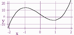
Using the graph we see that the roots are near \(\frac{1}{3}\), \(\frac{1}{2}\), and \(\frac{4}{3}\). We try synthetic division until we find that \(\frac{4}{3}\) is a root of the equation and that
\[6x^2 + 9x - 3\]
is the quotient of \(P(x)\) and \(x - \frac{4}{3}\).
We have
\[6x^2 + 9x - 3 = 3(2x^2 + 3x - 1).\]
Next we use the quadratic formula to find that the other two roots are
\[\dfrac{(-3 + \sqrt{17})}{4} \; \text{ and } \dfrac{ (-3-\sqrt{17})}{4}.\]
We can say that the factors are
\[x - \dfrac{3}{4}, x - \left[\dfrac{(-3 + \sqrt{17})}{4}\right], \; \text{and } x - \left[\dfrac{(-3 - \sqrt{17})}{4}\right].\]
Descartes' Rule of Signs
Theorem: Descartes' Rule of Signs
Let \(P(x)\) be a polynomial with real coefficients:
- The number of positive real roots either is equal to the number of variations in the sign of \(P(x)\) or is less then that by an even integer.
- The number of negative roots is either equal to the number of variations in the sign of \(P(-x)\) or is less than that by an even integer. Alternatively, to compute the number of negative roots, you change the sign of all the odd terms of \(P(x)\) and count the number of signs.
Example 4
Consider the function
\[f(x) = x^3 + 8x + 5.\]
Since all the signs are positive, there are no sign changes, hence there are no positive roots.
\[f(-x) = -x^3 - 8x + 5\]
We see one sign change hence there is exactly one negative real root. Therefore there must be two imaginary roots. Using synthetic division, we have that neither -5 nor -1 are roots, hence there are no rational roots. Since there is only one negative root, it cannot be of the form
\[a + b\sqrt{c}.\]
We can conclude that there is one irrational root that is not a square root, and two other roots \(a + bi\) and \(a - bi\).
Steps for finding roots:
- Use Descartes' rule of signs to determine positive and negative real roots.
- Use the \(\frac{p}{q}\) theorem (Rational Root Theorem) in coordination with Descartes' Rule of signs to find a possible roots.
- Plug in 1 and -1 to see if one of these two possibilities is a root. If so go to step 5.
- If not use synthetic division to test the other possibilities for roots until you find the first root. If there are no rational roots, give up or use a calculator.
- Find the quotient of dividing \(f(x)\) by \(x - r\).
- If the quotient is a quadratic, use the quadratic formula to find the last two roots. Otherwise go back to Step 2 applied to the quotient.
- Reread the question and answer it.
Exercises
- Find the rational zeros of each polynomial function
- Factor each over the set of integers
- \(x^3 + 7x^2 + 16x + 12\)
- \(2x^3 - 9x^2 + 14x - 10\)
- \(4x^4 - 28x^3 + 67x^2 - 63x + 18\)
- \(x^5 + x^4 - 6x^3 + 8x - 16\)
- Answer
-
For a worked out example, click here
Larry Green (Lake Tahoe Community College)
Integrated by Justin Marshall.


