4.9: The Intermediate Value Property

Definition: intermediate value property

A function \( f : A \rightarrow E ^ { * } \) is said to have the intermediate value property, or Darboux property, \( ^ { 1 } \) on a set \( B \subseteq A \) iff, together with any two function values \( f ( p ) \) and \( f \left( p _ { 1 } \right) \left( p , p _ { 1 } \in B \right) , \) it also takes all intermediate values between \( f ( p ) \) and \( f \left( p _ { 1 } \right) \) at some points of \( B \).

In other words, the image set \( f [ B ] \) contains the entire interval between \( f ( p ) \) and \( f \left( p _ { 1 } \right) \) in \( E ^ { * } . \)

Note 1. It follows that \( f [ B ] \) itself is a finite or infinite interval in \( E ^ { * } , \) with endpoints inf \( f [ B ] \) and \( \sup f [ B ] . \) (Verify!)

Geometrically, if \( A \subseteq E ^ { 1 } , \) this means that the curve \( y = f ( x ) \) meets all horizontal lines \( y = q , \) for \( q \) between \( f ( p ) \) and \( f \left( p _ { 1 } \right) . \) For example, in Figure 13 in \( § 1 , \) we have a "smooth" curve that cuts each horizontal line \( y = q \) between \( f ( 0 ) \) and \( f \left( p _ { 1 } \right) ; \) so \( f \) has the Darboux property on \( \left[ 0 , p _ { 1 } \right] . \) In Figures 14 and \( 15 , \) there is a "gap" at \( p \) ; the property fails. In Example (f) of \( § 1 , \) the property holds on all of \( E ^ { 1 } \) despite a discontinuity at \( 0 . \) Thus it does not imply continuity.

Intuitively, it seems plausible that a "continuous curve" must cut all intermediate horizontals. A precise proof for functions continuous on an interval, was given independently by Bolzano and Weierstrass (the same as in Theorem 2 of Chapter 3, §16). Below we give a more general version of Bolzano's proof based on the notion of a convex set and related concepts.

Definition: Convex

A set \( B \) in \( E ^ { n }\) (* or in another normed space) is said to be convex iff for each \( \overline { a } , \overline { b } \in B \) the line segment \( L [ \overline { a } , \overline { b } ] \) is a subset of \( B \).

A polygon joining \( \overline { a } \) and \( \overline { b } \) is any finite union of line segments (a "broken line") of the form

\[
\bigcup _ { i = 0 } ^ { m - 1 } L \left[ \overline { p } _ { i } , \overline { p } _ { i + 1 } \right] \text { with } \overline { p } _ { 0 } = \overline { a } \text { and } \overline { p } _ { m } = \overline { b }.
\]

The set \( B \) is said to be polygon connected (or piecewise convex) iff any two points \( \overline { a } , \overline { b } \in B \) can be joined by a polygon contained in \( B \).

Example

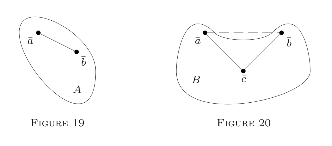
Any globe in \(E^{n}\) (* or in another normed space) is convex, so also is any interval in \(E^{n}\) or in \(E^{*}\). Figures 19 and 20 represent a convex set \(A\) and a polygon-connected set \(B\) in \(E^{2}\) is not convex; it has a "cavity").

We shall need a simple lemma that is noteworthy in its own right as well.

Lemma \(\PageIndex{1}\) (principle of nested line segments)

Every contracting sequence of closed line segments \(L\left[\overline{p}_{m}, \overline{q}_{m}\right]\) in \(E^{n}\) (* or in any other normed space) has a nonvoid intersection; i.e., there is a point

\[\overline{p} \in \bigcap_{m=1}^{\infty} L[\overline{p}_{m}, \overline{q}_{m}].\]

Proof

Use Cantor's theorem (Theorem 5 of §6) and Example (1) in §8. \(\square\)

We are now ready for Bolzano's theorem. The proof to be used is typical of so-called "bisection proofs." (See also §6, Problems 9 and 10 for such proofs.)

Theorem \(\PageIndex{1}\): Bolzano's theorem

If \(f : B \rightarrow E^{1}\) is relatively continuous on a polygon-connected set \(B\) in \(E^{n}\) (* or in another normed space), then \(f\) has the Darboux property on \(B .\)

In particular, if \(B\) is convex and if \(f(\overline{p})<c<f(\overline{q})\) for some \(\overline{p}, \overline{q} \in B,\) then there is a point \(\overline{r} \in L(\overline{p}, \overline{q})\) such that \(f(\overline{r})=c\).

Proof

First, let \(B\) be convex. Seeking a contradiction, suppose \(\overline{p}, \overline{q} \in B\) with

\[f(\overline{p})<c<f(\overline{q}),\]

yet \(f(\overline{x}) \neq c\) for all \(\overline{x} \in L(\overline{p}, \overline{q})\).

Let \(P\) be the set of all those \(\overline{x} \in L[\overline{p}, \overline{q}]\) for which \(f(\overline{x})<c,\) i.e.,

\[P=\{\overline{x} \in L[\overline{p}, \overline{q}] | f(\overline{x})<c\},\]

and let

\[Q=\{\overline{x} \in L[\overline{p}, \overline{q}] | f(\overline{x})>c\}.\]

Then \(\overline{p} \in P, \overline{q} \in Q, P \cap Q=\emptyset,\) and \(P \cup Q=L[\overline{p}, \overline{q}] \subseteq B\). (Why?)

Now let

\[\overline{r}_{0}=\frac{1}{2}(\overline{p}+\overline{q})\]

be the midpoint on \(L[\overline{p}, \overline{q}].\) Clearly, \(\overline{r}_{0}\) is either in \(P\) or in \(Q.\) Thus it bisects \(L[\overline{p}, \overline{q}]\) into two subsegments, one of which must have its left endpoint in \(P\) and its right endpoint in \(Q.\)

We denote this particular closed segment by \(L\left[\overline{p}_{1}, \overline{q}_{1}\right], \overline{p}_{1} \in P, \overline{q}_{1} \in Q.\) We then have

\[L[\overline{p}_{1}, \overline{q}_{1}] \subseteq L[\overline{p}, \overline{q}] \text { and }|p_{1}-q_{1}|=\frac{1}{2}|\overline{p}-\overline{q}|. \text { (Verify!) }\]

Now we bisect \(L[\overline{p}_{1}, \overline{q}_{1}]\) and repeat the process. Thus let

\[\overline{r}_{1}=\frac{1}{2}(\overline{p}_{1}+\overline{q}_{1}).\]

By the same argument, we obtain a closed subsegment \(L\left[\overline{p}_{2}, \overline{q}_{2}\right] \subseteq L\left[\overline{p}_{1}, \overline{q}_{1}\right]\) with \(\overline{p}_{2} \in P, \overline{q}_{2} \in Q,\) and

\[\left|\overline{p}_{2}-\overline{q}_{2}\right|=\frac{1}{2}\left|\overline{p}_{1}-\overline{q}_{1}\right|=\frac{1}{4}|\overline{p}-\overline{q}|.\]

Next, we bisect \(L\left[\overline{p}_{2}, \overline{q}_{2}\right],\) and so on. Continuing this process indefinitely, we obtain an infinite contracting sequence of closed line segments \(L\left[\overline{p}_{m}, \overline{q}_{m}\right]\) such that

\[(\forall m) \quad \overline{p}_{m} \in P, \overline{q}_{m} \in Q,\]

and

\[\left|\overline{p}_{m}-\overline{q}_{m}\right|=\frac{1}{2^{m}}|\overline{p}-\overline{q}| \rightarrow 0 \text { as } m \rightarrow+\infty.\]

By Lemma 1, there is a point

\[\overline{r} \in \bigcap_{m=1}^{\infty} L\left[\overline{p}_{m}, \overline{q}_{m}\right].\]

This implies that

\[(\forall m) \quad\left|\overline{r}-\overline{p}_{m}\right| \leq\left|\overline{p}_{m}-\overline{q}_{m}\right| \rightarrow 0,\]

whence \(\overline{p}_{m} \rightarrow \overline{r} .\) Similarly, we obtain \(\overline{q}_{m} \rightarrow \overline{r}\).

Now since \(\overline{r} \in L[\overline{p}, \overline{q}] \subseteq B,\) the function \(f\) is relatively continuous at \(\overline{r}\) over \(B\) (by assumption). By the sequential criterion, then,

\[f\left(\overline{p}_{m}\right) \rightarrow f(\overline{r}) \text { and } f\left(\overline{q}_{m}\right) \rightarrow f(\overline{r}).\]

Moreover, \(f\left(\overline{p}_{m}\right)<c<f\left(\overline{q}_{m}\right)\left(\text { for } \overline{p}_{m} \in P \text { and } \overline{q}_{m} \in Q\right) .\) Letting \(m \rightarrow+\infty,\) we pass to limits (Chapter 3, §15, Corollary 1 ) and get

\[f(\overline{r}) \leq c \leq f(\overline{r}),\]

so that \(\overline{r}\) is neither in \(P\) nor in \(Q,\) which is a contradiction. This completes the proof for a convex \(B\).

The extension to polygon-connected sets is left as an exercise (see Problem 2 below). Thus all is proved. \(\square\)

Note 2. In particular, the theorem applies if \(B\) is a globe or an interval.

Thus continuity on an interval implies the Darboux property. The converse fails, as we have noted. However, for monotone functions, we obtain the following theorem.

Theorem \(\PageIndex{2}\)

If a function \(f : A \rightarrow E^{1}\) is monotone and has the Darboux property on a finite or infinite interval \((a, b) \subseteq A \subseteq E^{1},\) then it is continuous on \((a, b).\)

Proof

Seeking a contradiction, suppose \(f\) is discontinuous at some \(p \in(a, b)\).

For definiteness, let \(f \uparrow\) on \((a, b) .\) Then by Theorems 2 and 3 in §5, we have either \(f\left(p^{-}\right)<f(p)\) or \(f(p)<f\left(p^{+}\right)\) or both, with no function values in between.

On the other hand, since \(f\) has the Darboux property, the function values \(f(x)\) for \(x\) in \((a, b)\) fill an entire interval (see Note 1). Thus it is impossible for \(f(p)\) to be the only function value between \(f\left(p^{-}\right)\) and \(f\left(p^{+}\right)\) unless \(f\) is constant near \(p,\) but then it is also continuous at \(p,\) which we excluded. This contradiction completes the proof. \(\square\)

Note 3. The theorem holds (with a similar proof) for nonopen intervals as well, but the continuity at the endpoints is relative (right at \(a,\) left at \(b).\)

Theorem \(\PageIndex{3}\)

If \(f : A \rightarrow E^{1}\) is strictly monotone and continuous when restricted to a finite or infinite interval \(B \subseteq A \subseteq E^{1},\) then its inverse \(f^{-1}\) has the same properties on the set \(f[B]\) (itself an interval, by Note 1 and Theorem 1).

Proof

It is easy to see that \(f^{-1}\) is increasing (decreasing) if \(f\) is; the proof is left as an exercise. Thus \(f^{-1}\) is monotone on \(f[B]\) if \(f\) is so on \(B\). To prove the relative continuity of \(f^{-1},\) we use Theorem 2, i.e., show that \(f^{-1}\) has the Darboux property on \(f[B].\)

Thus let \(f^{-1}(p)<c<f^{-1}(q)\) for some \(p, q \in f[B] .\) We look for an \(r \in f[B]\) such that \(f^{-1}(r)=c,\) i.e., \(r=f(c) .\) Now since \(p, q \in f[B],\) the numbers \(f^{-1}(p)\) and \(f^{-1}(q)\) are in \(B,\) an interval. Hence also the intermediate value \(c\) is in \(B\) ; thus it belongs to the domain of \(f,\) and so the function value \(f(c)\) exists. It thus suffices to put \(r=f(c)\) to get the result. \(\square\)

ExampleS

(a) Define \(f : E^{1} \rightarrow E^{1}\) by

\[f(x)=x^{n} \text { for a fixed } n \in N.\]

As \(f\) is continuous (being a monomial), it has the Darboux property on \(E^{1} .\) By Note \(1,\) setting \(B=[0,+\infty),\) we have \(f[B]=[0,+\infty)\). (Why?) Also, \(f\) is strictly increasing on \(B\). Thus by Theorem 3, the inverse function \(f^{-1}\) (i.e., the nth root function) exists and is continuous on \(f[B]=[0,+\infty)\).

If \(n\) is odd, then \(f^{-1}\) has these properties on all of \(E^{1},\) by a similar proof; thus \(\sqrt[n]{x}\) exists for \(x \in E^{1}\).

(b) Logarithmic functions. From the example in §5, we recall that the exponential function given by

\[F(x)=a^{x} \quad(a>0)\]

is continuous and strictly monotone on \(E^{1}.\) Its inverse, \(F^{-1},\) is called the logarithmic function to the base a, denoted log. By Theorem 3, it is continuous and strictly monotone on \(F\left[E^{1}\right].\)

To fix ideas, let \(a>1,\) so \(F \uparrow\) and \(\left(F^{-1}\right) \uparrow.\) By Note 1, \(F\left[E^{1}\right]\) is an interval with endpoints \(p\) and \(r,\) where

\[p=\inf F\left[E^{1}\right]=\inf \left\{a^{x} |-\infty<x<+\infty\right\}\]

and

\[r=\sup F\left[E^{1}\right]=\sup \left\{a^{x} |-\infty<x<+\infty\right\}.\]

Now by Problem 14 (iii) of §2 (with \(q=0\)),

\[\lim _{x \rightarrow+\infty} a^{x}=+\infty \text { and } \lim _{x \rightarrow-\infty} a^{x}=0.\]

As \(F \uparrow,\) we use Theorem 1 in §5 to obtain

\[r=\sup a^{x}=\lim _{x \rightarrow+\infty} a^{x}=+\infty \text { and } p=\lim _{x \rightarrow-\infty} a^{x}=0.\]

Thus \(F\left[E^{1}\right],\) i.e., the domain of \(\log _{a},\) is the interval \((p, r)=(0,+\infty)\). It follows that \(\log _{a} x\) is uniquely defined for \(x\) in \((0,+\infty) ;\) it is called the logarithm of \(x\) to the base \(a\).

The range of log \(_{a}\left(\text { i.e. of } F^{-1}\right)\) is the same as the domain of \(F,\) i.e., \(E^{1}\). Thus if \(a>1, \log _{a} x\) increases from \(-\infty\) to \(+\infty\) as \(x\) increases from 0 to \(+\infty.\) Hence

\[\lim _{x \rightarrow+\infty} \log _{a} x=+\infty \text { and } \lim _{x \rightarrow 0+} \log _{a} x=-\infty,\]

provided \(a>1\).

If \(0<a<1,\) the values of these limits are interchanged (since \(F \downarrow\) in this case), but otherwise the results are the same.

If \(a=e,\) we write \(\ln x\) or \(\log x\) for \(\log _{a} x,\) and we call \(\ln x\) the natural logarithm of \(x.\) Its inverse is, of course, the exponential \(f(x)=e^{x},\) also written \(\exp (x).\) Thus by definition, \(\ln e^{x}=x\) and

\[x=\exp (\ln x)=e^{\ln x} \quad(0<x<+\infty).\]

(c) The power function \(g :(0,+\infty) \rightarrow E^{1}\) is defined by

\[g(x)=x^{a} \text { for a fixed real } a.\]

If \(a>0,\) we also define \(g(0)=0.\) For \(x>0,\) we have

\[x^{a}=\exp \left(\ln x^{a}\right)=\exp (a \cdot \ln x).\]

Thus by the rules for composite functions (Theorem 3 and Corollary 2 in §2), the continuity of \(g\) on \((0,+\infty)\) follows from that of exponential and log functions. If \(a>0, g\) is also continuous at \(0.\) (Exercise!)