13.8: Laplace inverse

Up to now we have computed the inverse Laplace transform by table lookup. For example, $\mathcal{L}^{-1} (1/(s - a)) = e^{at}$. To do this properly we should first check that the Laplace transform has an inverse.

We start with the bad news: Unfortunately this is not strictly true. There are many functions with the same Laplace transform. We list some of the ways this can happen.

1. If $f(t) = g(t)$ for $t \ge 0$, then clearly $F(s) = G(s)$. Since the Laplace transform only concerns $t \ge 0$, the functions can differ completely for $t < 0$.
2. Suppose $f(t) = e^{at}$ and

$$g(t) = \begin{cases} f(t) & \text{ for } t \ne 1 \\ 0 & \text{ for } t = 1. \end{cases} \nonumber$$

That is, $f$ and $g$ are the same except we arbitrarily assigned them different values at $t = 1$. Then, since the integrals won’t notice the difference at one point, $F(s) = G(s) = 1/(s - a)$. In this sense it is impossible to define $\mathcal{L}^{-1} (F)$ uniquely.

The good news is that the inverse exists as long as we consider two functions that only differ on a negligible set of points the same. In particular, we can make the following claim.

Theorem $\PageIndex{1}$

Suppose $f$ and $g$ are continuous and $F(s) = G(s)$ for all $s$ with $\text{Re} (s) > a$ for some $a$. Then $f(t) = g(t)$ for $t \ge 0$.

This theorem can be stated in a way that includes piecewise continuous functions. Such a statement takes more care, which would obscure the basic point that the Laplace transform has a unique inverse up to some, for us, trivial differences.

We start with a few examples that we can compute directly.

Example $\PageIndex{1}$

Let

$$f(t) = e^{at}. \nonumber$$

So,

$$F(s) = \dfrac{1}{s - a}. \nonumber$$

Show

$$f(t) = \sum \text{Res} (F(s) e^{st}) \nonumber$$

$$f(t) = \dfrac{1}{2\pi i} \int_{c - i\infty}^{c + i \infty} F(s) e^{st}\ ds \nonumber$$

The sum is over all poles of $e^{st}/(s - a)$. As usual, we only consider $t > 0$.

Here, $c > \text{Re} (a)$ and the integral means the path integral along the vertical line $x = c$.

Solution

Proving Equation 13.8.4 is straightforward: It is clear that

$$\dfrac{e^{st}}{s -a} \nonumber$$

has only one pole which is at $s = a$. Since,

$$\sum \text{Res} (\dfrac{e^{st}}{s - a}, a) = e^{at} \nonumber$$

we have proved Equation 13.8.4.

Proving Equation 13.8.5 is more involved. We should first check the convergence of the integral. In this case, $s = c + iy$, so the integral is

$$\dfrac{1}{2\pi i} \int_{c - i \infty}^{c + i \infty} F(s) e^{st} \ ds = \dfrac{1}{2\pi i} \int_{-\infty}^{\infty} \dfrac{e^{(c + iy)t}}{c + iy - a} i \ dy = \dfrac{e^{ct}}{2 \pi} \int_{-\infty}^{\infty} \dfrac{e^{iyt}}{c + iy - a} \ dy. \nonumber$$

The (conditional) convergence of this integral follows using exactly the same argument as in the example near the end of Topic 9 on the Fourier inversion formula for $f(t) = e^{at}$. That is, the integrand is a decaying oscillation, around 0, so its integral is also a decaying oscillation around some limiting value.

Now we use the contour shown below.

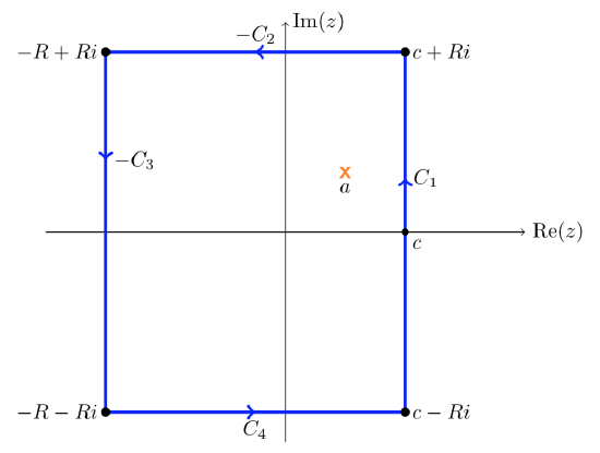
We will let $R$ go to infinity and use the following steps to prove Equation 13.8.5.

1. The residue theorem guarantees that if the curve is large enough to contain $a$ then
   $$\dfrac{1}{2\pi i} \int_{C_1 - C_2 - C_3 + C_4} \dfrac{e^{st}}{s - a}\ ds = \sum \text{Res} (\dfrac{e^{st}}{s - a}, a) = e^{at}. \nonumber$$
2. In a moment we will show that the integrals over $C_2, C_3, C_4$ all go to 0 as $R \to \infty$.
3. Clearly as $R$ goes to infinity, the integral over $C_1$ goes to the integral in Equation 13.8.5 Putting these steps together we have

$$e^{at} = \lim_{R \to \infty} \int_{C_1 - C_2 - C_3 + C_4} \dfrac{e^{st}}{s - a} \ ds = \int_{c - i\infty}^{c + i\infty} \dfrac{e^{st}}{s - a} \ ds \nonumber$$

Except for proving the claims in step 2, this proves Equation 13.8.5.

To verify step 2 we look at one side at a time.

$C_2$: $C_2$ is parametrized by $s = \gamma (u) = u + iR$, with $-R \le u \le c$. So,

$$|\int_{C_2} \dfrac{e^{st}}{s - a} \ ds| = \int_{-R}^{c} |\dfrac{e^{(u + iR)t}}{u + iR - a}| \le \int_{-R}^{c} \dfrac{e^{ut}}{R} \ du = \dfrac{e^{ct} - e^{-Rt}}{tR}. \nonumber$$

Since $c$ and $t$ are fixed, it’s clear this goes to 0 as $R$ goes to infinity.

The bottom $C_4$ is handled in exactly the same manner as the top $C_2$.

$C_3$: $C_3$ is parametrized by $s = \gamma (u) = -R + iu$, with $-R \le u \le R$. So,

$$|\int_{C_3} \dfrac{e^{st}}{s - a} \ ds| = \int_{-R}^{R} |\dfrac{e^{(-R + iu)t}}{-R + iu - a}| \le \int_{-R}^{R} \dfrac{e^{-Rt}}{R + a} \ du = \dfrac{e^{-Rt}}{R + a} \int_{-R}^{R} \ du = \dfrac{2\text{Re}^{-Rt}}{R+a}. \nonumber$$

Since $a$ and $t > 0$ are fixed, it’s clear this goes to 0 as $R$ goes to infinity.

Example $\PageIndex{2}$

Repeat the previous example with $f(t) = t$ for $t > 0$, $F(s) = 1/s^2$.

This is similar to the previous example. Since $F$ decays like $1/s^2$ we can actually allow $t \ge 0$

Theorem $\PageIndex{2}$ Laplace inversion 1

Assume $f$ is continuous and of exponential type $a$. Then for $c > a$ we have

$$f(t) = \dfrac{1}{2\pi i} \int_{c - i\infty}^{c + i\infty} F(s) e^{st}\ ds. \nonumber$$

As usual, this formula holds for $t > 0$.

Proof

The proof uses the Fourier inversion formula. We will just accept this theorem for now. Example 13.8.1 above illustrates the theorem.

Theorem $\PageIndex{3}$ Laplace inversion 2

Suppose $F(s)$ has a finite number of poles and decays like $1/s$ (or faster). Define

$$f(t) = \sum \text{Res} (F(s) e^{st}, p_k), \text{ where the sum is over all the poles } p_k. \nonumber$$

Then $\mathcal{L} (f; s) = F(s)$

Proof

Proof given in class. To be added here. The basic ideas are present in the examples above, though it requires a fairly clever choice of contours.

The integral inversion formula in Equation 13.8.13 can be viewed as writing $f(t)$ as a ‘sum’ of exponentials. This is extremely useful. For example, for a linear system if we know how the system responds to input $f(t) = e^{at}$ for all $a$, then we know how it responds to any input by writing it as a ‘sum’ of exponentials.