4.1: Basic Definitions

We shall now consider functions whose domains and ranges are sets in some fixed (but otherwise arbitrary) metric spaces $(S, \rho)$ and $\left(T, \rho^{\prime}\right),$ respectively. We write

$$f : A \rightarrow\left(T, \rho^{\prime}\right)$$

for a function $f$ with $D_{f}=A \subseteq(S, \rho)$ and $D_{f}^{\prime} \subseteq\left(T, \rho^{\prime}\right) . \quad S$ is called the domain space, and $T$ the range space, of $f .$

I. Given such a function, we often have to investigate its "local behavior" near some point $p \in S .$ In particular, if $p \in A=D_{f}(\text { so that } f(p) \text { is defined) we }$ may ask: Is it possible to make the function values $f(x)$ as near as we like ($" \varepsilon -$ near") to $f(p)$ by keeping $x$ sufficiently close $\left(\text { "close }^{\prime \prime}\right)$ to $p,$ i.e., inside some sufficiently small globe $G_{p}(\delta) ?$ If this is the case, we say that $f$ is continuous at $p .$ More precisely, we formulate the following definition.

Definition

A function $f : A \rightarrow\left(T, \rho^{\prime}\right),$ with $A \subseteq(S, \rho),$ is said to be continuous at $p$ iff $p \in A$ and, moreover, for each $\varepsilon>0$ (no matter how small) there is $\delta>0$ such that $\rho^{\prime}(f(x), f(p))<\varepsilon$ for all $x \in A \cap G_{p}(\delta) .$ In symbols,

$$(\forall \varepsilon>0)(\exists \delta>0)\left(\forall x \in A \cap G_{p}(\delta)\right)\left\{\begin{array}{l}{\rho^{\prime}(f(x), f(p))<\varepsilon, \text { or }} \\ {f(x) \in G_{f(p)}(\varepsilon)}\end{array}\right.$$

If $(1)$ fails, we say that $f$ is discontinuous at $p$ and call $p$ a discontinuity point of $f .$ This is also the case if $p \notin A$ (since $f(p)$ is not defined).

If $(1)$ holds for each p in a set $B \subseteq A,$ we say that $f$ is continuous on $B .$ If this is the case for $B=A,$ we simply say that $f$ is continuous.

Sometimes we prefer to keep $x$ near $p$ but different from $p .$ We then replace $G_{p}(\delta)$ in $(1)$ by the set $G_{p}(\delta)-\{p\},$ i.e., the globe without its center, denoted $G_{\neg p}(\delta)$ and called the deleted $\delta$ -globe about $p .$ This is even necessary if $p \notin D_{f}$. Replacing $f(p)$ in $(1)$ by some $q \in T,$ we then are led to the following definition.

Definition

Given $f : A \rightarrow\left(T, \rho^{\prime}\right), A \subseteq(S, \rho), p \in S,$ and $q \in T,$ we say that $f(x)$ tends to $q$ as $x$ tends to $p(f(x) \rightarrow q \text { as } x \rightarrow p)$ iff for each $\varepsilon>0$ there is $\delta>0$ such that $\rho^{\prime}(f(x), q)<\varepsilon$ for all $x \in A \cap G_{\neg p}(\delta) .$ In symbols,

$$(\forall \varepsilon>0)(\exists \delta>0)\left(\forall x \in A \cap G_{\neg p}(\delta)\right) \quad\left\{\begin{array}{l}{\rho^{\prime}(f(x), q)<\varepsilon, \text { i.e. }} \\ {f(x) \in G_{q}(\varepsilon)}\end{array}\right.$$

This means that $f(x)$ is $\varepsilon$ -close to $q$ when $x$ is $\delta$ -close to $p$ and $x \neq p$.

If $(2)$ holds for some $q,$ we call $q$ a limit of $f$ at $p .$ There may be no such $q$. We then say that $f$ has no limit at $p,$ or that this limit does not exist. If there is only one such $q(\text { for a given } p),$ we write $q=\lim _{x \rightarrow p} f(x) .$

Note 1. Formula (2) holds "vacuously" (see Chapter 1,8 §§1-3, end remark) if $A \cap G_{\neg p}(\delta)=\emptyset$ for some $\delta>0 .$ Then any $q \in T$ is a limit at $p,$ so a limit exists but is not unique. (We discard the case where $T$ is a singleton.)

Note 2. However, uniqueness is ensured if $A \cap G_{\neg p}(\delta) \neq \emptyset$ for all $\delta>0,$ as we prove below.

Observe that by Corollary 6 of Chapter 3, §14, the set $A$ clusters at $p$ iff

$$(\forall \delta>0) \quad A \cap G_{\neg p}(\delta) \neq \emptyset . \quad(\text { Explain! })$$

Thus we have the following corollary.

corollary $\PageIndex{1}$

If $A$ clusters at $p$ in $(S, \rho),$ then a function $f : A \rightarrow\left(T, p^{\prime}\right)$ can have at most one limit at $p ;$ i.e.

$$\lim _{x \rightarrow p} f(x) \text{ is unique (if it exists).}$$

In particular, this holds if $A \supseteq(a, b) \subset E^{1}(a<b)$ and $p \in[a, b]$.

Proof

Suppose $f$ has $t w o$ limits, $q$ and $r,$ at $p .$ By the Hausdorff property,

$$G_{q}(\varepsilon) \cap G_{r}(\varepsilon)=\emptyset \quad \text{ for some } \varepsilon>0.$$

Also, by $(2),$ there are $\delta^{\prime}, \delta^{\prime \prime}>0$ such that

$$\begin{array}{ll}{\left(\forall x \in A \cap G_{\neg p}\left(\delta^{\prime}\right)\right)} & {f(x) \in G_{q}(\varepsilon) \text { and }} \\ {\left(\forall x \in A \cap G_{\neg p}\left(\delta^{\prime \prime}\right)\right)} & {f(x) \in G_{r}(\varepsilon)}\end{array}$$

Let $\delta=\min \left(\delta^{\prime}, \delta^{\prime \prime}\right) .$ Then for $x \in A \cap G_{\neg p}(\delta), f(x)$ is in both $G_{q}(\varepsilon)$ and $G_{r}(\varepsilon)$, and such an $x$ exists since $A \cap G_{\neg p}(\delta) \neq \emptyset$ by assumption.

But this is impossible since $G_{q}(\varepsilon) \cap G_{r}(\varepsilon)=\emptyset$ $(\text { a contradiction!). } \square$

For intervals, see Chapter 3, §14, Example ( $\mathrm{h} )$.

corollary $\PageIndex{2}$

$f$ is continuous at $p\left(p \in D_{f}\right)$ iff $f(x) \rightarrow f(p)$ as $x \rightarrow p$.

Proof

The straightforward proof from definitions is left to the reader.

Note 3. In formula $(2),$ we excluded the case $x=p$ by assuming that $x \in A \cap G_{\neg p}(\delta) .$ This makes the behavior of $f$ at $p$ itself irrelevant. Thus for the existence of a limit $q$ at $p,$ it does not matter whether $p \in D_{f}$ or whether $f(p)=q .$ But both conditions are required for continuity at $p$ (see Corollary 2 and Definition 1$)$.

Note 4. Observe that if $(1)$ or $(2)$ holds for some $\delta,$ it certainly holds for any $\delta^{\prime} \leq \delta .$ Thus we may always choose $\delta$ as small as we like. Moreover, as $x$ is limited to $G_{p}(\delta),$ we may disregard, or change at will, the function values $f(x)$ for $x \notin G_{p}(\delta)$ ("local character of the limit notion").

II. Limits in E*. If $S$ or $T$ is $E^{*}\left(\text { or } E^{1}\right),$ we may let $x \rightarrow \pm \infty$ or $f(x) \rightarrow \pm \infty .$ For a precise definition, we rewrite $(2)$ in terms of $globes$ $G_{p}$ and $G_{q} :$

$$\left(\forall G_{q}\right)\left(\exists G_{p}\right)\left(\forall x \in A \cap G_{\neg p}\right) \quad f(x) \in G_{q}.$$

This makes sense also if $p=\pm \infty$ or $q=\pm \infty .$ We only have to use our conventions as to $G_{ \pm \infty},$ or the metric $\rho^{\prime}$ for $E^{*},$ as explained in Chapter 3, §11.

For example, consider

$$^{\prime \prime}f(x) \rightarrow q \text{ as } x \rightarrow+\infty^{\prime \prime}\left(A \subseteq S=E^{*}, p=+\infty, q \in\left(T, \rho^{\prime}\right)\right).$$

Here $G_{p}$ has the form $(a,+\infty], a \in E^{1},$ and $G_{\neg p}=(a,+\infty),$ while $G_{q}=G_{q}(\varepsilon)$, as usual. Noting that $x \in G_{\neg p}$ means $x>a\left(x \in E^{1}\right),$ we can rewrite $\left(2^{\prime}\right)$ as

$$(\forall \varepsilon>0)\left(\exists a \in E^{1}\right)(\forall x \in A | x>a) \quad f(x) \in G_{q}(\varepsilon), \text{ or } \rho^{\prime}(f(x), q)<\varepsilon.$$

This means that $f(x)$ becomes arbitrarily close to $q$ for large $x(x>a)$.

Next consider $^{4} f(x) \rightarrow+\infty$ as $x \rightarrow-\infty$ " Here $G_{\neg p}=(-\infty, a)$ and $G_{q}=(b,+\infty] .$ Thus formula $\left(2^{\prime}\right)$ yields (with $S=T=E^{*},$ and $x$ varying over $E^{\mathrm{i}} )$

$$\left(\forall b \in E^{1}\right)\left(\exists a \in E^{1}\right)(\forall x \in A | x<a) \quad f(x)>b;$$

similarly in other cases, which we leave to the reader.

Note 5. In $(3),$ we may take $A=N$ (the naturals). Then $f : N \rightarrow\left(T, \rho^{\prime}\right)$ is a sequence in $T .$ Writing $m$ for $x,$ set $u_{m}=f(m)$ and $a=k \in N$ to obtain

$$(\forall \varepsilon>0)(\exists k)(\forall m>k) \quad u_{m} \in G_{q}(\varepsilon) ; \text{ i.e., } \rho^{\prime}\left(u_{m}, q\right)<\varepsilon.$$

This coincides with our definition of the limit $q$ of a sequence $\left\{u_{m}\right\}$ (see Chapter 3, §14). Thus limits of sequences are a special case of function limits. Theorems on sequences can be obtained from those on functions $f : A \rightarrow\left(T, \rho^{\prime}\right)$ by simply taking $A=N$ and $S=E^{*}$ as above.

Note 6. Formulas $(3)$ and $(4)$ make sense sense also if $S=E^{1}$ (respectively, $S=T=E^{1} )$ since they do not involve any mention of $\pm \infty .$ We shall use such formulas also for functions $f : A \rightarrow T,$ with $A \subseteq S \subseteq E^{1}$ or $T \subseteq E^{1},$ as the case may be.

III. Relative Limits and Continuity. Sometimes the desired result $(1)$ or $(2)$ does not hold in full, but only with $A$ replaced by a smaller set $B \subseteq A$. Thus we may have

$$(\forall \varepsilon>0)(\exists \delta>0)\left(\forall x \in B \cap G_{\neg p}(\delta)\right) \quad f(x) \in G_{q}(\varepsilon).$$

In this case, we call $q$ a relative limit of $f$ at $p$ over $B$ and write

$$"f(x) \rightarrow q \text{ as } x \rightarrow p \text{ over } B"$$

or

$$\lim _{x \rightarrow p, x \in B} f(x)=q \quad(\text { if } q \text { is unique });$$

$B$ is called the path over which $x$ tends to $p .$ If, in addition, $p \in D_{f}$ and $q=f(p),$ we say that $f$ is relatively continuous at $p$ over $B ;$ then $(1)$ holds with $A$ replaced by $B$. Again, if this holds for every $p \in B,$ we say that $f$ is relatively continuous on $B .$ Clearly, if $B=A=D_{f},$ this yields ordinary (nonrelative) limits and continuity. Thus relative limits and continuity are more general.

Note that for limits over a path $B, x$ is chosen from $B$ or $B-\{p\}$ only. Thus the behavior of $f$ outside $B$ becomes irrelevant, and so we may arbitrarily redefine $f$ on $-B .$ For example, if $p \notin B$ but $\lim _{x \rightarrow p, x \in B} f(x)=q$ exists, we may define $f(p)=q,$ thus making $f$ relatively continuous at $p(\text { over } B) .$ We also may replace $(S, \rho)$ by $(B, \rho)(\text { if } p \in B),$ or restrict $f$ to $B,$ i.e., replace $f$ by the function $g : B \rightarrow\left(T, \rho^{\prime}\right)$ defined by $g(x)=f(x)$ for $x \in B$ (briefly, $g=f$ on $B )$.

A particularly important case is

$$A \subseteq S \subseteq E^{*}, \text{ e.g., } S=E^{1}.$$

Then inequalities are defined in $S,$ so we may take

$$B=\{x \in A | x<p\} \text{ (points in } A, \text{ preceding } p).$$

Then, writing $G_{q}$ for $G_{q}(\varepsilon)$ and $a=p-\delta,$ we obtain from formula $(2)$

$$\left(\forall G_{q}\right)(\exists a<p)(\forall x \in A | a<x<p) \quad f(x) \in G_{q}.$$

If $(5)$ holds, we call $q$ a left limit of $f$ at $p$ and write

$$"f(x) \rightarrow q \text{ as } x \rightarrow p^{-}" \quad\left(" x \text { tends to } p \text{ from the left}^{\prime}\right).$$

If, in addition, $q=f(p),$ we say that $f$ is left continuous at $p .$ Similarly, taking

$$B=\{x \in A | x>p\},$$

we obtain right limits and continuity. We write

$$f(x) \rightarrow q \text{ as } x \rightarrow p^{+}$$

iff $q$ is a right limit of $f$ at $p,$ i.e., if $(5)$ holds with all inequalities reversed.

If the set $B$ in question clusters at $p,$ the relative limit (if any) is unique. We then denote the left and right limit, respectively, by $f\left(p^{-}\right)$ and $f\left(p^{+}\right),$ and we write

$$\lim _{x \rightarrow p^{-}} f(x)=f\left(p^{-}\right) \text{ and } \lim _{x \rightarrow p^{+}} f(x)=f\left(p^{+}\right).$$

corollary $\PageIndex{3}$

With the previous notation, if $f(x) \rightarrow q$ as $x \rightarrow p$ over a path $B,$ and also over $D,$ then $f(x) \rightarrow q$ as $x \rightarrow p$ over $B \cup D$.

Hence if $D_{f} \subseteq E^{*}$ and $p \in E^{*},$ we have

$$q=\lim _{x \rightarrow p} f(x) \text{ iff } q=f\left(p^{-}\right)=f\left(p^{+}\right) . \quad(\text { Exercise! })$$

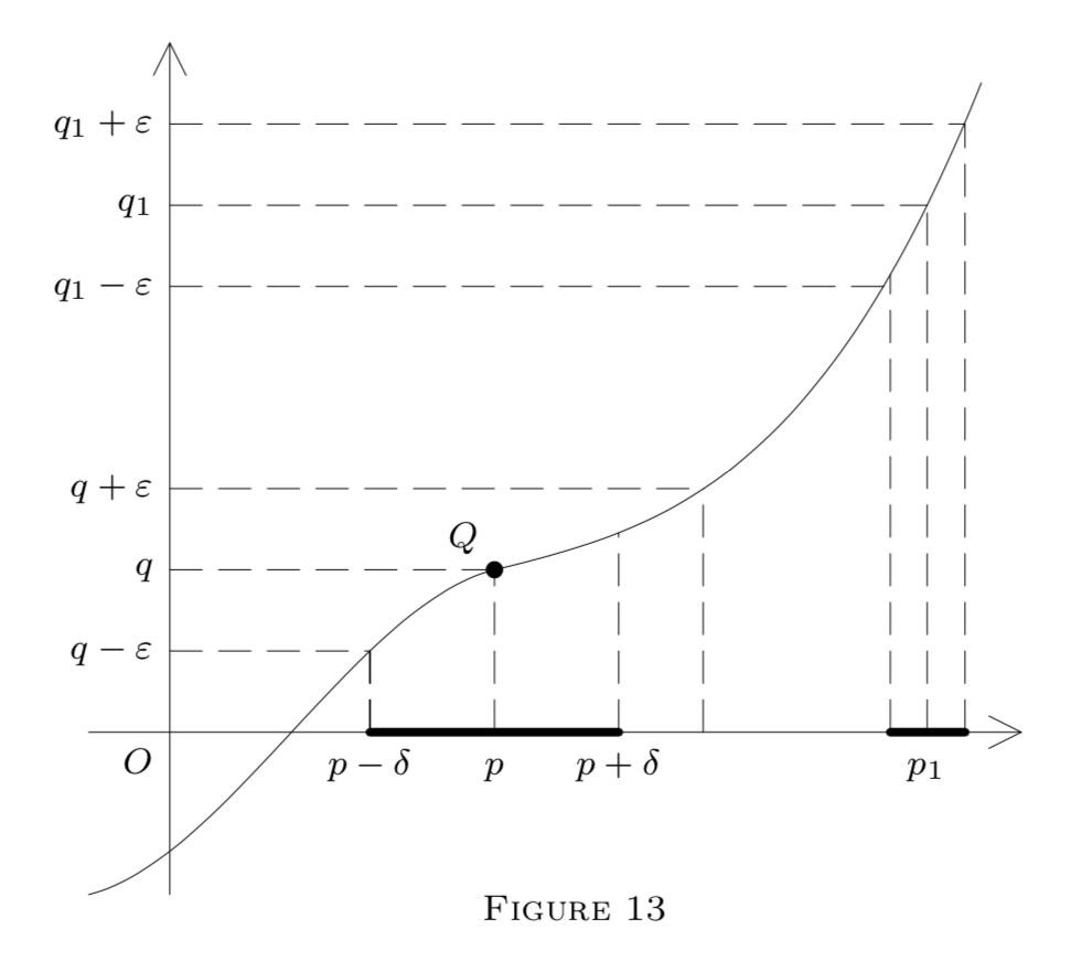
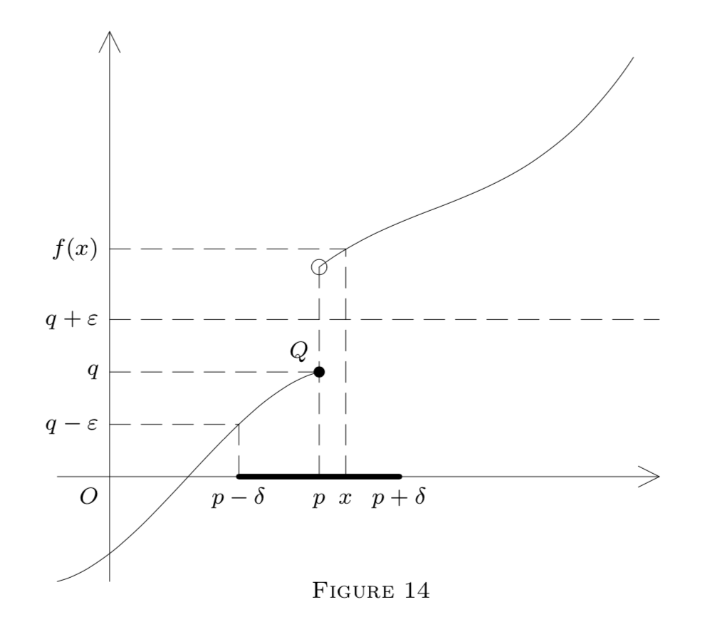
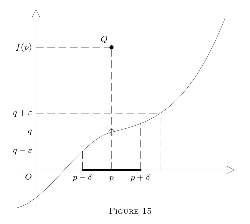
We now illustrate our definitions by a diagram in $E^{2}$ representing a function $f : E^{1} \rightarrow E^{1}$ by its graph, i.e., points $(x, y)$ such that $y=f(x)$.

Here

$$G_{q}(\varepsilon)=(q-\varepsilon, q+\varepsilon)$$

is an interval on the $y$ -axis. The dotted lines show how to construct an interval

$$(p-\delta, p+\delta)=G_{p}$$

on the $x$ -axis, satisfying formula $(1)$ in Figure $13,$ formulas $(5)$ and $(6)$ in Figure $14,$ or formula $(2)$ in Figure $15 .$ The point $Q$ in each diagram belongs to the graph; i.e., $Q=(p, f(p)) .$ In Figure $13, f$ is continuous at $p(\text { and also at }$ $p_{1}$ ). However, it is only left-continuous at $p$ in Figure $14,$ and it is discontinuous at $p$ in Figure $15,$ though $f\left(p^{-}\right)$ and $f\left(p^{+}\right)$ exist. (Why?)

Example $\PageIndex{1}$

(a) Let $f : A \rightarrow T$ be constant on $B \subseteq A ;$ i.e.

$$f(x)=q \text{ for a fixed } q \in T \text{ and all } x \in B.$$

Then $f$ is relatively continuous on $B,$ and $f(x) \rightarrow q$ as $x \rightarrow p$ over $B,$ at each $p .$ (Given $\varepsilon>0,$ take an arbitrary $\delta>0$. Then

$$\left(\forall x \in B \cap G_{\neg p}(\delta)\right) \quad f(x)=q \in G_{q}(\varepsilon),$$

as required; similarly for continuity.)

(b) Let $f$ be the $i$ dentity map on $A \subset(S, \rho) ;$ i.e.,

$$(\forall x \in A) \quad f(x)=x.$$

Then, given $\varepsilon>0,$ take $\delta=\varepsilon$ to obtain, for $p \in A$,

$$\left(\forall x \in A \cap G_{p}(\delta)\right) \quad \rho(f(x), f(p))=\rho(x, p)<\delta=\varepsilon.$$

Thus by $(1), f$ is continuous at any $p \in A,$ hence on $A$.

(c) Define $f : E^{1} \rightarrow E^{1}$ by

$$f(x)=1 \text{ if } x \text{ is rational, and } f(x)=0 \text{ otherwise.}$$

(This is the Dirichlet function, so named after Johann Peter Gustav Lejeune Dirichlet.)

No matter how small $\delta$ is, the globe

$$G_{p}(\delta)=(p-\delta, p+\delta)$$

(even the deleted globe) contains both rationals and irrationals. Thus as $x$ varies over $G_{\neg p}(\delta), f(x)$ takes on both values, 0 and $1,$ many times and so gets out of any $G_{q}(\varepsilon),$ with $q \in E^{1}, \varepsilon<\frac{1}{2}$.

Hence for any $q, p \in E^{1},$ formula $(2)$ fails if we take $\varepsilon=\frac{1}{4},$ say. Thus $f$ has no limit at any $p \in E^{1}$ and hence is discontinuous everywhere! However, $f$ is relatively continuous on the set $R$ of all rationals by Example $(\mathrm{a})$.

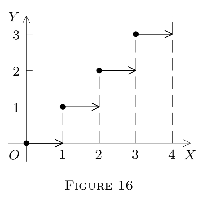
(d) Define $f : E^{1} \rightarrow E^{1}$ by

$$f(x)=[x](=\text { the integral part of } x ; \text { see Chapter } 2, §10).$$

Thus $f(x)=0$ for $x \in[0,1), f(x)=1$ for $x \in[1,2),$ etc. Then $f$ is discontinuous at $p$ if $p$ is an integer (why?) but continuous at any other $p\left(\text { restrict } f \text { to a small } G_{p}(\delta) \text { so as to make it constant) }\right.$

However, left and right limits exist at each $p \in E^{1},$ even if $p=$ $n(\text { an integer }) .$ In fact,

$$f(x)=n, x \in(n, n+1)$$

and

$$f(x)=n-1, x \in(n-1, n),$$

hence $f\left(n^{+}\right)=n$ and $f\left(n^{-}\right)=$ $n-1 ; f$ is right continuous on $E^{1} .$ See Figure $16 .$

(e) Define $f : E^{1} \rightarrow E^{1}$ by

$$f(x)=\frac{x}{|x|} \text{ if } x \neq 0, \text{ and } f(0)=0.$$

(This is the so-called signum function, often denoted by sgn.)

Then (Figure 17$)$

$$f(x)=-1 \text{ if } x<0$$

and

$$f(x)=1 \text{ if } x>0.$$

Thus, as in ( d ), we infer that $f$ is discontinuous at $0,$ but continuous at each $p \neq 0 .$ Also, $f\left(0^{+}\right)=1$ and $f\left(0^{-}\right)=-1 .$ Redefining $f(0)=1$ or $f(0)=-1,$ we can make $f$ right (respectively, left) continuous at $0,$ but not both.

(f) Define $f : E^{1} \rightarrow E^{1}$ by (see Figure 18$)$

$$f(x)=\sin \frac{1}{x} \text{ if } x \neq 0, \text{ and } f(0)=0.$$

Any globe $G_{0}(\delta)$ about 0 contains points at which $f(x)=1,$ as well as those at which $f(x)=-1$ or $f(x)=0$ (take $x=2 /(n \pi)$ for large integers $n )$; in fact, the graph "oscillates" infinitely many times between $-1$ and $1 .$ Thus by the same argument as in $(\mathrm{c}), f$ has no limit at 0 (not even a left or right limit) and hence is discontinuous at $0 .$ No attempt at redefining $f$ at 0 can restore even left or right continuity, let alone ordinary continuity, at $0 .$

(g) Define $f : E^{2} \rightarrow E^{1} \mathrm{by}$

$$f(\overline{0})=0 \text{ and } f(\overline{x})=\frac{x_{1} x_{2}}{x_{1}^{2}+x_{2}^{2}} \text{ if } \overline{x}=\left(x_{1}, x_{2}\right) \neq \overline{0}.$$

Let $B$ be any line in $E^{2}$ through $\overline{0},$ given parametrically by

$$\overline{x}=t \vec{u}, \quad t \in E^{1}, \vec{u} \text{ fixed (see Chapter 3, §§4-6 ),}$$

so $x_{1}=t u_{1}$ and $x_{2}=t u_{2} .$ As is easily seen, for $\overline{x} \in B, f(\overline{x})=f(\overline{u})$ (constant) if $\overline{x} \neq \overline{0} .$ Hence

$$\left(\forall \overline{x} \in B \cap G_{\neg \overline{0}}(\delta)\right) \quad f(\overline{x})=f(\overline{u}),$$

i.e., $\rho(f(\overline{x}), f(\overline{u}))=0<\varepsilon,$ for any $\varepsilon>0$ and any deleted globe about $\overline{0}$.

By $\left(2^{\prime}\right),$ then, $f(\overline{x}) \rightarrow f(\overline{u})$ as $\overline{x} \rightarrow \overline{0}$ over the path $B .$ Thus $f$ has a relative limit $f(\overline{u})$ at $\overline{0},$ over any line $\overline{x}=t \overline{u},$ but this limit is different for various choices of $\overline{u},$ i.e., for different lines through $\overline{0} .$ No ordinary limit at $\overline{0}$ exists (why?); $f$ is not even relatively continuous at $\overline{0}$ over the line $\overline{x}=t \vec{u}$ unless $f(\overline{u})=0$ (which is the case only if the line is one of the coordinate axes (why?)).