4.2: Maximization By The Simplex Method

Learning Objectives

In this section, you will learn to solve linear programming maximization problems using the Simplex Method:

1. Identify and set up a linear program in standard maximization form
2. Convert inequality constraints to equations using slack variables
3. Set up the initial simplex tableau using the objective function and slack equations
4. Find the optimal simplex tableau by performing pivoting operations.
5. Identify the optimal solution from the optimal simplex tableau.

In the last chapter, we used the geometrical method to solve linear programming problems, but the geometrical approach will not work for problems that have more than two variables. In real life situations, linear programming problems consist of literally thousands of variables and are solved by computers. We can solve these problems algebraically, but that will not be very efficient. Suppose we were given a problem with, say, 5 variables and 10 constraints. By choosing all combinations of five equations with five unknowns, we could find all the corner points, test them for feasibility, and come up with the solution, if it exists. But the trouble is that even for a problem with so few variables, we will get more than 250 corner points, and testing each point will be very tedious. So we need a method that has a systematic algorithm and can be programmed for a computer. The method has to be efficient enough so we wouldn't have to evaluate the objective function at each corner point. We have just such a method, and it is called the simplex method.

The simplex method was developed during the Second World War by Dr. George Dantzig. His linear programming models helped the Allied forces with transportation and scheduling problems. In 1979, a Soviet scientist named Leonid Khachian developed a method called the ellipsoid algorithm which was supposed to be revolutionary, but as it turned out it is not any better than the simplex method. In 1984, Narendra Karmarkar, a research scientist at AT&T Bell Laboratories developed Karmarkar's algorithm which has been proven to be four times faster than the simplex method for certain problems. But the simplex method still works the best for most problems.

The simplex method uses an approach that is very efficient. It does not compute the value of the objective function at every point; instead, it begins with a corner point of the feasibility region where all the main variables are zero and then systematically moves from corner point to corner point, while improving the value of the objective function at each stage. The process continues until the optimal solution is found.

To learn the simplex method, we try a rather unconventional approach. We first list the algorithm, and then work a problem. We justify the reasoning behind each step during the process. A thorough justification is beyond the scope of this course.

We start out with an example we solved in the last chapter by the graphical method. This will provide us with some insight into the simplex method and at the same time give us the chance to compare a few of the feasible solutions we obtained previously by the graphical method. But first, we list the algorithm for the simplex method.

THE SIMPLEX METHOD

1. Set up the problem. That is, write the objective function and the inequality constraints.
2. Convert the inequalities into equations. This is done by adding one slack variable for each inequality.
3. Construct the initial simplex tableau. Write the objective function as the bottom row.
4. The most negative entry in the bottom row identifies the pivot column.
5. Calculate the quotients. The smallest quotient identifies a row. The element in the intersection of the column identified in step 4 and the row identified in this step is identified as the pivot element. The quotients are computed by dividing the far right column by the identified column in step 4. A quotient that is a zero, or a negative number, or that has a zero in the denominator, is ignored.
6. Perform pivoting to make all other entries in this column zero. This is done the same way as we did with the Gauss-Jordan method.
7. When there are no more negative entries in the bottom row, we are finished; otherwise, we start again from step 4.
8. Read off your answers. Get the variables using the columns with 1 and 0s. All other variables are zero. The maximum value you are looking for appears in the bottom right hand corner.

Now, we use the simplex method to solve Example 3.1.1 solved geometrically in section 3.1.

Example \(\PageIndex{1}\)

Niki holds two part-time jobs, Job I and Job II. She never wants to work more than a total of 12 hours a week. She has determined that for every hour she works at Job I, she needs 2 hours of preparation time, and for every hour she works at Job II, she needs one hour of preparation time, and she cannot spend more than 16 hours for preparation. If she makes $40 an hour at Job I, and $30 an hour at Job II, how many hours should she work per week at each job to maximize her income?

Solution

In solving this problem, we will follow the algorithm listed above.

STEP 1. Set up the problem. Write the objective function and the constraints.

Since the simplex method is used for problems that consist of many variables, it is not practical to use the variables \(x\), \(y\), \(z\) etc. We use symbols \(x_1\), \(x_2\), \(x_3\), and so on.

Let

• \(x_1\) = The number of hours per week Niki will work at Job I and
• \(x_2\) = The number of hours per week Niki will work at Job II.

It is customary to choose the variable that is to be maximized as \(Z\).

The problem is formulated the same way as we did in the last chapter.

\[\begin{array}{ll}
\textbf { Maximize } & \mathrm{Z}=40 \mathrm{x}_{1}+30 \mathrm{x}_{2} \\
\textbf { Subject to: } & \mathrm{x}_{1}+\mathrm{x}_{2} \leq 12 \\
& 2 \mathrm{x}_{1}+\mathrm{x}_{2} \leq 16 \\
& \mathrm{x}_{1} \geq 0 ; \mathrm{x}_{2} \geq 0
\end{array}\nonumber \]

STEP 2. Convert the inequalities into equations. This is done by adding one slack variable for each inequality.

For example to convert the inequality \(x_1 + x_2 ≤ 12\) into an equation, we add a non-negative variable \(y_1\), and we get

\[x_1 + x_2 + y_1 = 12 \nonumber \]

Here the variable \(y_1\) picks up the slack, and it represents the amount by which \(x_1 + x_2\) falls short of 12. In this problem, if Niki works fewer than 12 hours, say 10, then \(y_1\) is 2. Later when we read off the final solution from the simplex table, the values of the slack variables will identify the unused amounts.

We rewrite the objective function \(Z = 40x_1 + 30x_2\) as \(- 40x_1 - 30x_2 + Z = 0\).

After adding the slack variables, our problem reads

\[\begin{array}{ll}
\text { Objective function } & - 40x_1 - 30x_2 + Z = 0 \\
\text { Subject to constraints: } & x_1 + x_2 + y_1 = 12 \\
& 2x_1 + x_2 + y_2 = 16 \\
& x1 ≥ 0; x2 ≥ 0
\end{array} \nonumber \]

STEP 3. Construct the initial simplex tableau. Each inequality constraint appears in its own row. (The non-negativity constraints do not appear as rows in the simplex tableau.) Write the objective function as the bottom row.

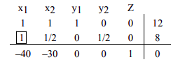
Now that the inequalities are converted into equations, we can represent the problem into an augmented matrix called the initial simplex tableau as follows.

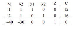
Here the vertical line separates the left hand side of the equations from the right side. The horizontal line separates the constraints from the objective function. The right side of the equation is represented by the column C.

The reader needs to observe that the last four columns of this matrix look like the final matrix for the solution of a system of equations. If we arbitrarily choose \(x_1 = 0\) and \(x_2 = 0\), we get

\[\left[\begin{array}{ccccc}
y_{1} & y_{2} & Z & | & C \\
1 & 0 & 0 & | & 12 \\
0 & 1 & 0 & | & 16 \\
0 & 0 & 1 & | & 0
\end{array}\right]\nonumber \]

which reads

\[y_1 = 12 \quad y_2 = 16 \quad Z = 0 \nonumber \]

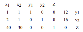
The solution obtained by arbitrarily assigning values to some variables and then solving for the remaining variables is called the basic solution associated with the tableau. So the above solution is the basic solution associated with the initial simplex tableau. We can label the basic solution variable in the right of the last column as shown in the table below.

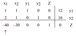
STEP 4. The most negative entry in the bottom row identifies the pivot column.

The most negative entry in the bottom row is -40; therefore the column 1 is identified.

Question Why do we choose the most negative entry in the bottom row?

Answer The most negative entry in the bottom row represents the largest coefficient in the objective function - the coefficient whose entry will increase the value of the objective function the quickest.

The simplex method begins at a corner point where all the main variables, the variables that have symbols such as \(x_1\), \(x_2\), \(x_3\) etc., are zero. It then moves from a corner point to the adjacent corner point always increasing the value of the objective function. In the case of the objective function \(Z = 40x_1+ 30x_­2\), it will make more sense to increase the value of \(x_1\) rather than \(x_2\). The variable \(x_1\) represents the number of hours per week Niki works at Job I. Since Job I pays $40 per hour as opposed to Job II which pays only $30, the variable \(x_1\) will increase the objective function by $40 for a unit of increase in the variable \(x_1\).

STEP 5. Calculate the quotients. The smallest quotient identifies a row. The element in the intersection of the column identified in step 4 and the row identified in this step is identified as the pivot element.

Following the algorithm, in order to calculate the quotient, we divide the entries in the far right column by the entries in column 1, excluding the entry in the bottom row.

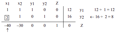
The smallest of the two quotients, 12 and 8, is 8. Therefore row 2 is identified. The intersection of column 1 and row 2 is the entry 2, which has been highlighted. This is our pivot element.

Question Why do we find quotients, and why does the smallest quotient identify a row?

Answer When we choose the most negative entry in the bottom row, we are trying to increase the value of the objective function by bringing in the variable \(x_1\). But we cannot choose any value for \(x_1\). Can we let \(x_1 = 100\)? Definitely not! That is because Niki never wants to work for more than 12 hours at both jobs combined: \(x_1 + x_2 ≤ 12\). Can we let \(x_1 = 12\)? Again, the answer is no because the preparation time for Job I is two times the time spent on the job. Since Niki never wants to spend more than 16 hours for preparation, the maximum time she can work is 16 ÷ 2 = 8.

Now you see the purpose of computing the quotients; using the quotients to identify the pivot element guarantees that we do not violate the constraints.

Question Why do we identify the pivot element?

Answer As we have mentioned earlier, the simplex method begins with a corner point and then moves to the next corner point always improving the value of the objective function. The value of the objective function is improved by changing the number of units of the variables. We may add the number of units of one variable, while throwing away the units of another. Pivoting allows us to do just that.

The variable whose units are being added is called the entering variable, and the variable whose units are being replaced is called the departing variable. The entering variable in the above table is \(x_1\), and it was identified by the most negative entry in the bottom row. The departing variable \(y_2\) was identified by the lowest of all quotients.

STEP 6. Perform pivoting to make all other entries in this column zero.

In chapter 2, we used pivoting to obtain the row echelon form of an augmented matrix. Pivoting is a process of obtaining a 1 in the location of the pivot element, and then making all other entries zeros in that column. So now our job is to make our pivot element a 1 by dividing the entire second row by 2. The result follows.

To obtain a zero in the entry first above the pivot element, we multiply the second row by -1 and add it to row 1. We get

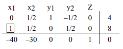
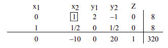
To obtain a zero in the element below the pivot, we multiply the second row by 40 and add it to the last row.

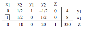
We now determine the basic solution associated with this tableau. By arbitrarily choosing \(x_2 = 0\) and \(y_2 = 0\), we obtain \(x_1 = 8\), \(y_1 = 4\), and \(z = 320\). If we write the augmented matrix, whose left side is a matrix with columns that have one 1 and all other entries zeros, we get the following matrix stating the same thing.

\[\left[\begin{array}{ccccc}
\mathrm{x}_{1} & \mathrm{y}_1 & \mathrm{Z} & | & \mathrm{C} \\
0 & 1 & 0 & | & 4 \\
1 & 0 & 0 & | & 8 \\
0 & 0 & 1 & | & 320
\end{array}\right] \nonumber \]

We can restate the solution associated with this matrix as \(x_1 = 8\), \(x_2 = 0\), \(y_1 = 4\), \(y_2 = 0\) and \(z = 320\). At this stage of the game, it reads that if Niki works 8 hours at Job I, and no hours at Job II, her profit Z will be $320. Recall from Example 3.1.1 in section 3.1 that (8, 0) was one of our corner points. Here \(y_1 = 4\) and \(y_2 = 0\) mean that she will be left with 4 hours of working time and no preparation time.

STEP 7. When there are no more negative entries in the bottom row, we are finished; otherwise, we start again from step 4.

Since there is still a negative entry, -10, in the bottom row, we need to begin, again, from step 4. This time we will not repeat the details of every step, instead, we will identify the column and row that give us the pivot element, and highlight the pivot element. The result is as follows.

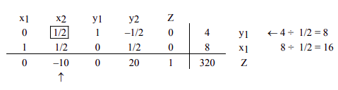
We make the pivot element 1 by multiplying row 1 by 2, and we get

Now to make all other entries as zeros in this column, we first multiply row 1 by -1/2 and add it to row 2, and then multiply row 1 by 10 and add it to the bottom row.

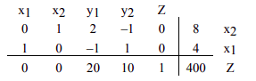
We no longer have negative entries in the bottom row, therefore we are finished.

Question Why are we finished when there are no negative entries in the bottom row?

Answer The answer lies in the bottom row. The bottom row corresponds to the equation:

\[\begin{array}{l}
0 x_{1}+0 x_{2}+20 y_{1}+10 y_{2}+Z=400 \quad \text { or } \\
z=400-20 y 1-10 y 2
\end{array}\nonumber \]

Since all variables are non-negative, the highest value \(Z\) can ever achieve is 400, and that will happen only when \(y_1\) and \(y_2\) are zero.

STEP 8. Read off your answers.

We now read off our answers, that is, we determine the basic solution associated with the final simplex tableau. Again, we look at the columns that have a 1 and all other entries zeros. Since the columns labeled \(y_1\) and \(y_2\) are not such columns, we arbitrarily choose \(y_1 = 0\), and \(y_2 = 0\), and we get

\[\left[\begin{array}{ccccc}
\mathrm{x}_{1} & \mathrm{x}_{2} & \mathrm{Z} & | & \mathrm{C} \\
0 & 1 & 0 & | & 8 \\
1 & 0 & 0 & | & 4 \\
0 & 0 & 1 & | & 400
\end{array}\right] \nonumber \]

The matrix reads \(x_1 = 4\), \(x_2= 8\) and \(z = 400\).

The final solution says that if Niki works 4 hours at Job I and 8 hours at Job II, she will maximize her income to $400. Since both slack variables are zero, it means that she would have used up all the working time, as well as the preparation time, and none will be left.

­