18.5: Mean-Field Approximation on Random Networks

If we can assume that the network topology is random with connection probability $p_e$, then infection occurs with a joint probability of three events: that a node is connected to another neighbor node ($p_e$), that the neighbor node is infected by the disease $(q)$, and that the disease is actually transmitted to the node ($p_i$). Therefore, $1−p_{e}qp_{i}$ is the probability that the node is not infected by another node. In order for a susceptible node to remain susceptible to the next time step, it must avoid infection in this way $n−1$ times, i.e., for all other nodes in the network. The probability for this to occur is thus (\(1 − p_{e}qp_{i})^{n−1}. Using this result, all possible scenarios of state transitions can be summarized as shown in Table 18.5.1.

Table $\PageIndex{1}$: Possible scenarios of state transitions in the network SIS model.

Current state	Next state	Probabiltiy of this transition
0 (susceptible)	0 (suceptible)	$$(1-q)(1-p_{e}qp_{i})^{n-1} \nonumber$$
0 (susceptible)	1 (infected)	$$(1-q)(1-(1-p_{e}qp_{i})^{n-1}) \nonumber$$
1 (infected)	0 (susceptible)	$$qp_{r} \nonumber$$
1 (infected)	1 (infected)	$$q(1-p_{r}) \nonumber$$

We can combine the probabilities of the transitions that turn the next state into 1, to write the following difference equation for $q_{t}$ (whose subscript is omitted on the right hand side for simplicity):

$$\begin{align} q_{t+1} = (1-q)(1-(1-p_{e}qp_{i})^{n-1}) q(1-p_{r})\label{(18.19)} \\ = 1-q-(1-q)(1-p_{e}qp_{i})^{n-1} +q-qp_{r} \label{18.20} \\ \approx 1-(1-q)(1-(n-1)p_{e}qp_{i})-qp_{r} \label{(18.21)} \qquad{ (because \ p_{e}qp_{i} \ is \ small)} \\ =q((1-q)(n-1)p_{e}p_{i} +1 -p_{r}) \label{(18.22)} \\ = q((1-q)s+1-p_{r}) =f(q) \qquad{(with \ s = (n-1)p_{e}p_{i})} \label{(18.23)} \end{align}$$

Now this is a simple iterative map about qt, which we already know how to study. By solving $f(q_{eq}) = q_{eq}$, we can easily find that there are the following two equilibrium points:

$$q_{eq} =0, 1-\frac{p_{r}}{s} \label{(18.24)}$$

And the stability of each of these points can be studied by calculating the derivative of $f(q)$:

$$\frac{df(q)}{dq}=1-p_{r}+(1-2q)s \label{(18.25)}$$

$$\frac{df(q)}{dq}|_{q=0} =1-p_{r}+s \label{(18.26)}$$
$$\frac{df(q)}{dq}|_{q=1-p_{r}/s} =1+p_{r}-s \label{(18.27)}$$

So, it looks like $p_r −s$ is playing an important role here. Note that $0 ≤ p_{r} ≤ 1$ because it is a probability, and also $0 ≤ s ≤ 1$ because $(1−s)$ is an approximation of ($1−p_{e}qp_{i})n−1$, which is also a probability. Therefore, the valid range of $p_r −s$ is between -1 and 1. By comparing the absolute values of Eqs. $\ref{(18.26)}$ and $\ref{(18.27)}$ to 1 within this range, we find the stabilities of those two equilibrium points as summarized in Table 18.5.2.

Table $\PageIndex{2}$: Stabilities of the two equilibrium points in the network SIS model.

Equilibrium point	$$-1 \leq{ p_{r}-s} \leq{0} \nonumber$$	$$0< p_{r}-s \leq{1} \nonumber$$
$$q=0 \nonumber$$	unstable	stable
$$q=1 -\frac{P_{r}}{s} \nonumber$$	stable	unstable

Now we know that there is a critical epidemic threshold between the two regimes. If $p_r > s = (n−1)p_{e}p_{i}$, the equilibrium point $q_{eq} = 0$ becomes stable, so the disease should go away quickly. But otherwise, the other equilibrium point becomes stable instead, which means that the disease will never go away from the network. This epidemic threshold is often written in terms of the infection probability, as

$$p_{i} > \frac{p_{r}}{(n-1)p_{e}} =\frac{p_{r}}{\langle {k}\rangle} \label{(18.28)}$$

as a condition for the disease to persist, where $\langle{k}\rangle$ is the average degree. It is an important characteristic of epidemic models on random networks that there is a positive lower bound for the disease’s infection probability. In other words, a disease needs to be “contagious enough” in order to survive in a randomly connected social network.

Exercise $\PageIndex{1}$

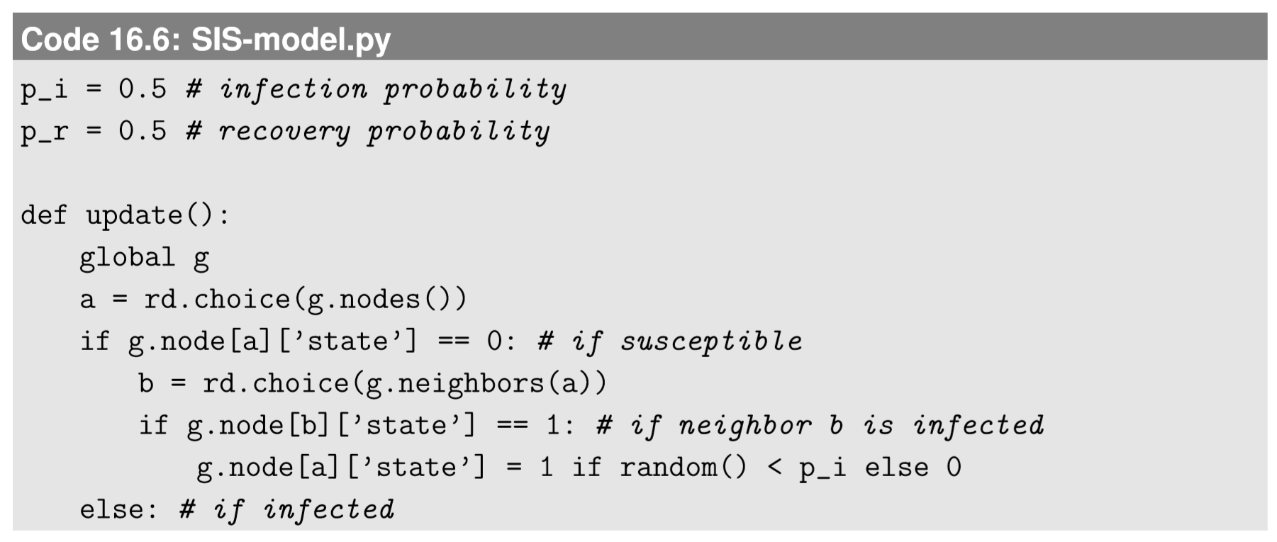
Modify Code 16.6 to implement a synchronous, simultaneous updating version of the network SIS model. Then simulate its dynamics on an Erd˝osR´enyi random network for the following parameter settings:

• n = 100, $p_{e} = 0.1$, $p_{i} = 0.5$, $p_{r} = 0.5 (pr < (n−1)p_{e}p_{i})$

• n = 100, $p_e = 0.1$, $p_i = 0.04$, $p_r = 0.5 (p_r > (n−1)p_ep_i)$

• n = 200, $p_e = 0.1$, $p_i = 0.04$, $p_r = 0.5 (p_r < (n−1)p_ep_i)$

• n = 200, $p_e = 0.05$, $p_i = 0.04$, $p_r = 0.5 (p_r > (n−1)p_ep_i)$

Discuss how the results compare to the predictions made by the mean-field approximation.

As you can see in the exercise above, the mean-field approximation works much better on random networks than on CA. This is because the topologies of random networks are not locally clustered. Edges connect nodes that are randomly chosen from the entire network, so each edge serves as a global bridge to mix the states of the system, effectively bringing the system closer to the “mean-field” state. This, of course, will break down if the network topology is not random but locally clustered, such as that of the Watts-Strogatz small-world networks. You should keep this limitation in mind when you apply mean-field approximation.

Exercise $\PageIndex{2}$

If you run the simulation using the original Code 16.6 with asynchronous updating, the result may be different from the one obtained with synchronous updating. Conduct simulations using the original code for the same parameter settings as those used in the previous exercise. Compare the results obtained using the two versions of the model, and discuss why they are so different.