
18.1: Dynamics of Continuous-State Networks


- Last updated
- Apr 30, 2024
- Save as PDF

( \newcommand{\kernel}{\mathrm{null}\,}\)
We will now switch gears to the analysis of dynamical properties of networks. We will first discuss how some of the analytical techniques we already covered in earlier chapters can be applied to dynamical network models, and then we will move onto some additional topics that are specific to networks.
First of all, I would like to make it clear that we were already discussing dynamical network models in earlier chapters. A typical autonomous discrete-time dynamical system
xt=F(xt−1)
or a continuous-time one
dxdt=F(x),
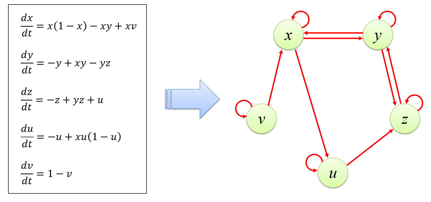
can be considered a dynamical network if the state space is multidimensional. For example, a system with a five-dimensional state space can be viewed as a dynamical network made of five nodes, each having a scalar state that changes dynamically based on the mathematical rule determined in function F (Fig. 18.1). More specifically, the dynamics of node i’s state is determined by the i-th dimensional part of F, and if that part refers to the state vector’s j-th component, then node j is connected to node i, and so on.
This means that dynamical networks are not fundamentally different from other dynamical systems. Therefore, if the node states are continuous, then all the analytical
techniques we discussed before—finding equilibrium points, linearizing dynamics around an equilibrium point, analyzing the stability of the system’s state using eigenvalues of a Jacobian matrix, etc.—will apply to dynamical network models without any modification.
Analysis of dynamical networks is easiest when the model is linear, i.e.,
xt=Axt−1
or
dxdt=Ax
If this is the case, all you need to do is to find eigenvalues of the coefficient matrix A, identify the dominant eigenvalue(s) λd (with the largest absolute value for discrete-time cases, or the largest real part for continuous-time cases), and then determine the stability of the system’s state around the origin by comparing |λd|_with1fordiscrete−timecases,or\(Re(λd) with 0 for continuous-time cases. The dominant eigenvector(s) that correspond to λd also tell us the asymptotic state of the network. While this methodology doesn’t apply to other more general nonlinear network models, it is still quite useful, because many important network dynamics can be written as linear models. One such example is diffusion, which we will discuss in the following section in more detail.