Search

Text Color

Margin Size

Font Type

Enable Dyslexic Font

12.10: Trees

Last updated

Jan 2, 2025
Save as PDF
- 12.9.1: Exercises
- 12.10.1: Exercises

$\newcommand{\vecs}[1]{\overset { \scriptstyle \rightharpoonup} {\mathbf{#1}} }$

$\newcommand{\vecd}[1]{\overset{-\!-\!\rightharpoonup}{\vphantom{a}\smash {#1}}}$

$\newcommand{\id}{\mathrm{id}}$ $\newcommand{\Span}{\mathrm{span}}$

( \newcommand{\kernel}{\mathrm{null}\,}\) $\newcommand{\range}{\mathrm{range}\,}$

$\newcommand{\RealPart}{\mathrm{Re}}$ $\newcommand{\ImaginaryPart}{\mathrm{Im}}$

$\newcommand{\Argument}{\mathrm{Arg}}$ $\newcommand{\norm}[1]{\| #1 \|}$

$\newcommand{\inner}[2]{\langle #1, #2 \rangle}$

$\newcommand{\Span}{\mathrm{span}}$

$\newcommand{\id}{\mathrm{id}}$

$\newcommand{\Span}{\mathrm{span}}$

$\newcommand{\kernel}{\mathrm{null}\,}$

$\newcommand{\range}{\mathrm{range}\,}$

$\newcommand{\RealPart}{\mathrm{Re}}$

$\newcommand{\ImaginaryPart}{\mathrm{Im}}$

$\newcommand{\Argument}{\mathrm{Arg}}$

$\newcommand{\norm}[1]{\| #1 \|}$

$\newcommand{\inner}[2]{\langle #1, #2 \rangle}$

$\newcommand{\Span}{\mathrm{span}}$ $\newcommand{\AA}{\unicode[.8,0]{x212B}}$

$\newcommand{\vectorA}[1]{\vec{#1}} % arrow$

$\newcommand{\vectorAt}[1]{\vec{\text{#1}}} % arrow$

$\newcommand{\vectorB}[1]{\overset { \scriptstyle \rightharpoonup} {\mathbf{#1}} }$

$\newcommand{\vectorC}[1]{\textbf{#1}}$

$\newcommand{\vectorD}[1]{\overrightarrow{#1}}$

$\newcommand{\vectorDt}[1]{\overrightarrow{\text{#1}}}$

$\newcommand{\vectE}[1]{\overset{-\!-\!\rightharpoonup}{\vphantom{a}\smash{\mathbf {#1}}}}$

$\newcommand{\vecs}[1]{\overset { \scriptstyle \rightharpoonup} {\mathbf{#1}} }$

$\newcommand{\vecd}[1]{\overset{-\!-\!\rightharpoonup}{\vphantom{a}\smash {#1}}}$

$\newcommand{\avec}{\mathbf a}$

$\newcommand{\bvec}{\mathbf b}$

$\newcommand{\cvec}{\mathbf c}$

$\newcommand{\dvec}{\mathbf d}$

$\newcommand{\dtil}{\widetilde{\mathbf d}}$

$\newcommand{\evec}{\mathbf e}$

$\newcommand{\fvec}{\mathbf f}$

$\newcommand{\nvec}{\mathbf n}$

$\newcommand{\pvec}{\mathbf p}$

$\newcommand{\qvec}{\mathbf q}$

$\newcommand{\svec}{\mathbf s}$

$\newcommand{\tvec}{\mathbf t}$

$\newcommand{\uvec}{\mathbf u}$

$\newcommand{\vvec}{\mathbf v}$

$\newcommand{\wvec}{\mathbf w}$

$\newcommand{\xvec}{\mathbf x}$

$\newcommand{\yvec}{\mathbf y}$

$\newcommand{\zvec}{\mathbf z}$

$\newcommand{\rvec}{\mathbf r}$

$\newcommand{\mvec}{\mathbf m}$

$\newcommand{\zerovec}{\mathbf 0}$

$\newcommand{\onevec}{\mathbf 1}$

$\newcommand{\real}{\mathbb R}$

$\newcommand{\twovec}[2]{\left[\begin{array}{r}#1 \\ #2 \end{array}\right]}$

$\newcommand{\ctwovec}[2]{\left[\begin{array}{c}#1 \\ #2 \end{array}\right]}$

$\newcommand{\threevec}[3]{\left[\begin{array}{r}#1 \\ #2 \\ #3 \end{array}\right]}$

$\newcommand{\cthreevec}[3]{\left[\begin{array}{c}#1 \\ #2 \\ #3 \end{array}\right]}$

$\newcommand{\fourvec}[4]{\left[\begin{array}{r}#1 \\ #2 \\ #3 \\ #4 \end{array}\right]}$

$\newcommand{\cfourvec}[4]{\left[\begin{array}{c}#1 \\ #2 \\ #3 \\ #4 \end{array}\right]}$

$\newcommand{\fivevec}[5]{\left[\begin{array}{r}#1 \\ #2 \\ #3 \\ #4 \\ #5 \\ \end{array}\right]}$

$\newcommand{\cfivevec}[5]{\left[\begin{array}{c}#1 \\ #2 \\ #3 \\ #4 \\ #5 \\ \end{array}\right]}$

$\newcommand{\mattwo}[4]{\left[\begin{array}{rr}#1 \amp #2 \\ #3 \amp #4 \\ \end{array}\right]}$

$\newcommand{\laspan}[1]{\text{Span}\{#1\}}$

$\newcommand{\bcal}{\cal B}$

$\newcommand{\ccal}{\cal C}$

$\newcommand{\scal}{\cal S}$

$\newcommand{\wcal}{\cal W}$

$\newcommand{\ecal}{\cal E}$

$\newcommand{\coords}[2]{\left\{#1\right\}_{#2}}$

$\newcommand{\gray}[1]{\color{gray}{#1}}$

$\newcommand{\lgray}[1]{\color{lightgray}{#1}}$

$\newcommand{\rank}{\operatorname{rank}}$

$\newcommand{\row}{\text{Row}}$

$\newcommand{\col}{\text{Col}}$

$\renewcommand{\row}{\text{Row}}$

$\newcommand{\nul}{\text{Nul}}$

$\newcommand{\var}{\text{Var}}$

$\newcommand{\corr}{\text{corr}}$

$\newcommand{\len}[1]{\left|#1\right|}$

$\newcommand{\bbar}{\overline{\bvec}}$

$\newcommand{\bhat}{\widehat{\bvec}}$

$\newcommand{\bperp}{\bvec^\perp}$

$\newcommand{\xhat}{\widehat{\xvec}}$

$\newcommand{\vhat}{\widehat{\vvec}}$

$\newcommand{\uhat}{\widehat{\uvec}}$

$\newcommand{\what}{\widehat{\wvec}}$

$\newcommand{\Sighat}{\widehat{\Sigma}}$

$\newcommand{\lt}{<}$

$\newcommand{\gt}{>}$

$\newcommand{\amp}{&}$

$\definecolor{fillinmathshade}{gray}{0.9}$

A row of trees with no leaves. — Figure $\PageIndex{1}$ : In graph theory, graphs known as trees have structures in common with live trees. (credit: “Row of trees in Roslev” by AKA CJ/Flickr, Public Domain)

Learning Objectives

Describe and identify trees.
Determine a spanning tree for a connected graph.
Find the minimum spanning tree for a weighted graph.
Solve application problems involving trees.

We saved the best for last! In this last section, we will discuss arguably the most fun kinds of graphs, trees. Have you every researched your family tree? Family trees are a perfect example of the kind of trees we study in graph theory. One of the characteristics of a family tree graph is that it never loops back around, because no one is their own grandparent!

What Is A Tree?

Whether we are talking about a family tree or a tree in a forest, none of the branches ever loops back around and rejoins the trunk. This means that a tree has no cyclic subgraphs, or is acyclic. A tree also has only one component. So, a tree is a connected acyclic graph. Here are some graphs that have the same characteristic. Each of the graphs in Figure $\PageIndex{2}$ is a tree.

Three graphs. Graph T has 15 vertices. The edges are as follows: a b, b c, c d, c i, i j, j k, k o, d e, d l, e n, e m, b f, f g, and g h. Graph P has 6 vertices. The edges are as follows: t s, s r, r q, q p, and p o. Graph S has 7 vertices. The edges are as follows: u t, u v, u w, u x, u y, and u z. — Figure $\PageIndex{2}$ : Graphs T, P, and S

Let’s practice determining whether a graph is a tree. To do this, check if a graph is connected and has no cycles.

Example $\PageIndex{1}$ : Identifying Trees

Identify any trees in Figure $\PageIndex{3}$ . If a graph is not a tree, explain how you know.

Three graphs. Graph M has 7 vertices. The edges are a b, b f, f g, f c, b c, b d, and d e. Graph N has 6 vertices. The edges are I j, I h, l k, and l m. The edges, I j, and l k intersect each other. Graph P has 6 vertices. The edges are s t, s r, r q, q p, and p o. — Figure $\PageIndex{3}$ : Graphs M, N, and P

Answer

Graph M is not a tree because it contains the cycle (b, c, f).
Graph N is not a tree because it is not connected. It has two components, one with vertices h, i, j, and another with vertices k, l, m.
Graph P is a tree. It has no cycles and it is connected.

Your Turn $\PageIndex{1}$

There are some configurations that are commonly used when setting up computer networks. Several of them are shown in the given figure. Which of the configurations in the figure appear to have the characteristics of a tree graph? If a configuration does not appear to have the characteristics of a tree graph, explain how you know.

Four illustrations represent the common network configurations. The first illustration represents mesh topology. Six computers are interconnected. The second illustration represents a ring topology. Five computers are connected in a ring. The third illustration represents star topology. A computer at the center is connected to five computers surrounding it. The fourth illustration represents tree topology. Two branches arise from a horizontal bus. Each branch has a computer at the center connected to five computers surrounding it — Figure $\PageIndex{4}$ : Common Network Configurations

Types of Trees

Mathematicians have had a lot of fun naming graphs that are trees or that contain trees. For example, the graph in Figure $\PageIndex{5}$ is not a tree, but it contains two components, one containing vertices a through d, and the other containing vertices e through g, each of which would be a tree on its own. This type of structure is called a forest. There are also interesting names for trees with certain characteristics.

A path graph or linear graph is a tree graph that has exactly two vertices of degree 1 such that the only other vertices form a single path between them, which means that it can be drawn as a straight line.
A star tree is a tree that has exactly one vertex of degree greater than 1 called a root, and all other vertices are adjacent to it.
A starlike tree is a tree that has a single root and several paths attached to it.
A caterpillar tree is a tree that has a central path that can have vertices of any degree, with each vertex not on the central path being adjacent to a vertex on the central path and having a degree of one.
A lobster tree is a tree that has a central path that can have vertices of any degree, with paths consisting of either one or two edges attached to the central path.

Examples of each of these types of structures are given in Figure $\PageIndex{6}$ .

Graph F has 8 vertices. The vertices are labeled a to h. Edges connect b a, b d, b c, f e, f h, and f g. — Figure $\PageIndex{5}$ : Forest Graph F

Six graphs. Graph S has 7 vertices. The edges are a b, b f, f g, f c, b c, b d, and d e. Graph N has 6 vertices. The edges are I j, I h, l k, and l m. The edges, I j, and l k intersect each other. Graph P has 6 vertices. The edges are s t, s r, r q, q p, and p o. Graph Z has 12 vertices. The edges are a b, a c, a d, a e, a f, a g, a h, h i, c j, e k, and k l. Graph C has 14 vertices. The edges are m n, n z, n o, o r, o p, o x, o y, p y, p x, p s, p t, p u, p q, p v, and p w. Graph L has 26 vertices. The edges are f q, f t, f s, f e, e o, e p, p z, e d, d m, m v, d n, n y, d c, c k, k u, c l, l k, c b, b i, i t, b j, j w, b a, b g, and b h. — Figure $\PageIndex{6}$ : Six Types of Trees

Example $\PageIndex{2}$ : Identifying Types of Trees

Each graph in Figure $\PageIndex{7}$ is one of the special types of trees we have been discussing. Identify the type of tree.

Two graphs. Graph U has 17 vertices. The edges are o q, o p, o l, l n, l k, l m, l i, I j, I f, f g, f h, f d, d e, f b, b c, and b a. Graph V hs 6 vertices. The edges are r s, s t, t u, u v, and v w. The edges, s t and u v intersect. — Figure $\PageIndex{7}$ Graphs U and V

Answer

Graph U has a central path a → b → d → f → i → l → o → q. Each vertex that is not on the path has degree 1 and is adjacent to a vertex that is on the path. So, U is a caterpillar tree.

Graph V is a path graph because it is a single path connecting exactly two vertices of degree one, r → s → u → v → w.

Your Turn $\PageIndex{2}$

Of the network configurations from Figure $\PageIndex{7}$ , which, if any, has the characteristics of a

Star tree?
Caterpillar tree?
Path graph?

Characteristics of Trees

As we study trees, it is helpful to be familiar with some of their characteristics. For example, if you add an edge to a tree graph between any two existing vertices, you will create a cycle, and the resulting graph is no longer a tree. Some examples are shown in Figure $\PageIndex{8}$ . Adding edge bj to Graph T creates cycle (b, c, i, j). Adding edge rt to Graph P creates cycle (r, s, t). Adding edge tv to Graph S creates cycle (t, u, v).

Three graphs. Graph T has 15 vertices. The edges are as follows: a b, b c, c d, c i, i j, j k, k o, d e, d l, e n, e m, b f, f g, and g h. The edges, c i, and i j are in blue. A dashed edge connects b and j. Graph P has 6 vertices. The edges are as follows: t s, s r, r q, q p, and p o. The edges, t s, and s r are in blue. A dashed edge connects t and r. Graph S has 7 vertices. The edges are as follows: u t, u v, u w, u x, u y, and u z. The edges, u t, and u v are in blue. A dashed edge connects t and v. — Figure $\PageIndex{8}$ : Adding Edges to Trees

It is also true that removing an edge from a tree graph will increase the number of components and the graph will no longer be connected. In fact, you can see in Figure \(\PageIndex{8}\ that removing one or more edges can create a forest. Removing edge qr from Graph P creates a graph with two components, one with vertices o, p and q, and the other with vertices r, s, and t. Removing edge uw from Graph S creates two components, one with just vertex w and the other with the rest of the vertices. When two edges were removed from Graph T, edge bf and edge cd, creates a graph with three components as shown in Figure $\PageIndex{9}$ .

Three graphs. Graph T has 15 vertices. The edges are as follows: a b, b c, c d, c i, i j, j k, k o, d e, d l, e n, e m, b f, f g, and g h. The edges, d c, and b f are in dashed lines. The graph is separated into three blocks. Graph P has 6 vertices. The edges are as follows: t s, s r, r q, q p, and p o. The edge, q r is in dashed lines. The graph is separated into two blocks. Graph S has 7 vertices. The edges are as follows: u t, u v, u w, u x, u y, and u z. The edge, u w is in dashed lines. The graph is separated into two blocks. — Figure $\PageIndex{9}$ : Removing Edges from Trees

A very useful characteristic of tree graphs is that the number of edges is always one less than the number of vertices. In fact, any connected graph in which the number of edges is one less than the number of vertices is guaranteed to be a tree. Some examples are given in Figure $\PageIndex{10}$ .

Six graphs. Graph T has 15 vertices. The edges are as follows: a b, b c, c d, c i, i j, j k, k o, d e, d l, e n, e m, b f, f g, and g h. Graph P has 6 vertices. The edges are as follows: t s, s r, r q, q p, and p o. Graph S has 7 vertices. The edges are as follows: u t, u v, u w, u x, u y, and u z. Graph Z has 12 vertices. The edges are a b, a c, a d, a e, a f, a g, a h, h i, c j, e k, and k l. Graph C has 14 vertices. The edges are m n, n z, n o, o r, o p, o x, o y, p y, p x, p s, p t, p u, p q, p v, and p w. Graph L has 26 vertices. The edges are f q, f t, f s, f e, e o, e p, p z, e d, d m, m v, d n, n y, d c, c k, k u, c l, l k, c b, b i, i t, b j, j w, b a, b g, and b h. — Figure $\PageIndex{10}$ : Number of Vertices and Edges in Trees vs. Other Graphs

FORMULA

The number of edges in a tree graph with $n$ vertices is $n - 1$ .

A connected graph with n vertices and $n - 1$ edges is a tree graph.

Example $\PageIndex{3}$ : Exploring Characteristics of Trees

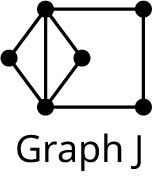
Use Graphs I and J in Figure $\PageIndex{11}$ to answer each question.

Two graphs. Graph I has six vertices: a, b, c, d, e, and f. Edges connect a b, b c, b e, d e, and e f. Graph J has seven vertices: g h, i, j, k, l, and m. Edges connect g h, h i, j h, j l, k l, and l m.

Figure

$\PageIndex{11}$ Graphs I and J

Which vertices are in each of the components that remain when edge be is removed from Graph I?
Determine the number of edges and the number of vertices in Graph J. Explain how this confirms that Graph J is a tree.
What kind of cycle is created if edge im is added to Graph J?

Answer

When edge be is removed, there are two components that remain. One component includes vertices a, b, and c. The other component includes vertices d, e, and f.
There are seven vertices and six edges in Graph J. This confirms that Graph J is a tree because the number of edges is one less than the number of vertices.
The pentagon (i, h, j, l, m) is created when edge im is added to Graph J.

Your Turn $\PageIndex{3}$

Use Graphs I and J in Figure $\PageIndex{11}$ to answer each question.

Which vertices are in each of the components that remain when edge jl is removed from Graph J?

Determine the number of edges and the number of vertices in Graph I. Explain how this confirms that Graph I is a tree.

What kind of cycle is created if edge cf is added to Graph I?

Who Knew?: Graph Theory in the Movies

In the 1997 film Good Will Hunting, the main character, Will, played by Matt Damon, solves what is supposed to be an exceptionally difficult graph theory problem, “Draw all the homeomorphically irreducible trees of size $n =$ 10n=10.” That sounds terrifying! But don’t panic. Watch this great Numberphile video to see why this is actually a problem you can do at home!

Video

The Problem in Good Will Hunting by Numberphile

Spanning Trees

Suppose that you planned to set up your own computer network with four devices. One option is to use a “mesh topology” like the one in Figure $\PageIndex{12}$ , in which each device is connected directly to every other device in the network.

The mesh topology for four devices could be represented by the complete Graph A₁ in Figure $\PageIndex{13}$ where the vertices represent the devices, and the edges represent network connections. However, the devices could be networked using fewer connections. Graphs A₂, A_3, and A₄ of Figure $\PageIndex{13}$ show configurations in which three of the six edges have been removed. Each of the Graphs A₂, A₃ and A₄ in Figure 12.242 is a tree because it is connected and contains no cycles. Since Graphs A₂, A₃ and A₄ are also subgraphs of Graph A₁ that include every vertex of the original graph, they are also known as spanning trees.

Four graphs. Graph A 1 has four vertices: a, b, c, and d. The edges are a b, b d, d c, c a, a d, and b c. Graph A 2 has four vertices: a, b, c, and d. The edges are a b, b c, and c d. Graph A 3 has four vertices: a, b, c, and d. The edges are a b, a c, and c d. Graph A 4 has four vertices: a, b, c, and d. The edges are a b, a c, and a d. — Figure $\PageIndex{13}$ : Network Configurations for Four Devices

By definition, spanning trees must span the whole graph by visiting all the vertices. Since spanning trees are subgraphs, they may only have edges between vertices that were adjacent in the original graph. Since spanning trees are trees, they are connected and they are acyclic. So, when deciding whether a graph is a spanning tree, check the following characteristics:

All vertices are included.
No vertices are adjacent that were not adjacent in the original graph.
The graph is connected.
There are no cycles.

Example $\PageIndex{4}$ 9: Identifying Spanning Trees

Use Figure $\PageIndex{14}$ to determine which of graphs M₁, M₂, M₃, and M₄, are spanning trees of Q.

Five graphs. Graph Q has six vertices: a, b, c, d, e, and f. The edges are a b, a c, a d, b d, d f, c d, c e, c f, and e f. Graph M 1 has six vertices: a, b, c, d, e, and f. The edges are a b, b d, d c, c e, f, and f d. Graph M 2 has six vertices: a, b, c, d, e, and f. The edges are a b, a d, d f, f e, and e c. Graph M 3 has six vertices; a, b, c, d, e, and f. The edges are b d, d f, a f, f e, and e c. Graph M 4 has six vertices: a, b, c, d, e, and f. The edges are a b, c e, e f, and f d. — Figure $\PageIndex{14}$ Graphs Q, M₁, M₂, M_3, and M₄

Answer

Graph M₁ is not a spanning tree of Graph Q because it has a cycle (c, d, f, e).
Graph M₂ is a spanning tree of Graph Q because it has all the original vertices, no vertices are adjacent in M₂ that weren’t adjacent in Graph Q, Graph M₂ is connected and it contains no cycles.
Graph M₃ is not a spanning tree of Graph Q because vertices a and f are adjacent in Graph M₃ but not in Graph Q.
Graph M₄ is not a spanning tree of Graph Q because it is not connected.

So, only graph M₂ is a spanning tree of Graph Q.

Your Turn $\PageIndex{4}$

Use the given figure for the following exercises.

Five graphs. Graph H has five vertices: n, q, r, s, and t. The edges are p q, p r, q r, q t, r t, r s, and s t. Graph N 1 has four vertices: p, q, s, and t. The edges are p t, q s, and s t. Graph N 2 has five vertices: p, q, r, s, and t. The edges are p r, q r, r s, r t, and s t. Graph N 3 has five vertices: p, q, r, s, and t. The edges are p q, q r, r s, and qt. Graph N 4 has five vertices: p, q, r, s, and t. The edges are p q, r s, and s t. — Figure $\PageIndex{15}$

1. Since sq is not an edge in Graph H, Graph N₁ cannot be a spanning tree of H.

True
False

2. Graph N₂ is a spanning tree of Graph H.

True
False

3. Graph N₃ is a spanning tree of Graph H.

True
False

4. Since there is no path between p and t in Graph N₄, it cannot be a spanning tree of any graph.

True
False

Constructing a Spanning Tree Using Paths

Suppose that you wanted to find a spanning tree within a graph. One approach is to find paths within the graph. You can start at any vertex, go any direction, and create a path through the graph stopping only when you can’t continue without backtracking as shown in Figure $\PageIndex{16}$ .

A graph with 23 vertices and 35 edges. Ten edges are highlighted in green. Two vertices are labeled started here and stopped here. — Figure $\PageIndex{16}$ : First Phase to Construct a Spanning Tree

Once you have stopped, pick a vertex along the path you drew as a starting point for another path. Make sure to visit only vertices you have not visited before as shown in Figure $\PageIndex{17}$ .

A graph with 23 vertices and 35 edges. Ten edges are highlighted in blue. Ten edges are highlighted in green. Two vertices are labeled started here and stopped here. — Figure $\PageIndex{17}$ : Intermediate Phase to Construct a Spanning Tree

Repeat this process until all vertices have been visited as shown in Figure $\PageIndex{18}$ .

The end result is a tree that spans the entire graph as shown in Figure $\PageIndex{19}$ .

A graph with 23 vertices and 22 edges. — Figure $\PageIndex{19}$ : The Resulting Spanning Tree

Notice that this subgraph is a tree because it is connected and acyclic. It also visits every vertex of the original graph, so it is a spanning tree. However, it is not the only spanning tree for this graph. By making different turns, we could create any number of distinct spanning trees.

Example $\PageIndex{5}$ : Constructing Spanning Trees

Construct two distinct spanning trees for the graph in Figure $\PageIndex{20}$ .

Graph L has 11 vertices and 19 edges. The graph resembles a square resting below a triangle on either side. The triangles are connected via a trapezoid. The squares have diagonal lines. — Figure $\PageIndex{20}$ Graph L

Answer: Two possible solutions are given in Figure $\PageIndex{21}$ and Figure $\PageIndex{22}$ .

$Two graphs depict removing edges from graph L. The first graph has 11 vertices and 19 edges. It resembles a square resting below a triangle on either side. The triangles are connected via a trapezoid. The squares have diagonal lines. 6 edges are in green, 2 edges are in purple, and 2 edges are in blue. Green represents phase 1, blue represents phase 2, and purple represents phase 3. The second graph is the final tree. The black edges from the first graph are removed.$
Figure $\PageIndex{21}$ First Spanning Tree for Graph L

$Two graphs depict removing edges from graph L. The first graph has 11 vertices and 19 edges. It resembles a square resting below a triangle on either side. The triangles are connected via a trapezoid. The squares have diagonal lines. 6 edges are in green, 2 edges are in purple, and 2 edges are in blue. Green represents phase 1, blue represents phase 2, and purple represents phase 3. The second graph is the final tree. The black edges from the first graph are removed.$
Figure $\PageIndex{22}$ : Second Spanning Tree for Graph L

Your Turn $\PageIndex{5}$

Construct three distinct spanning trees for Graph J.

Graph J has 6 vertices and 8 edges. — Figure $\PageIndex{23}$ : Graph J

Revealing Spanning Trees

Another approach to finding a spanning tree in a connected graph involves removing unwanted edges to reveal a spanning tree. Consider Graph D in Figure $\PageIndex{24}$ .

Graph D has 10 vertices. The vertices are labeled from a to j. The edges are c d, c a, d a, a g, a h, g h, a b, b e, b f, e f, b i, b j, and I j. — Figure $\PageIndex{24}$ : Graph D

Graph D has 10 vertices. A spanning tree of Graph D must have 9 edges, because the number of edges is one less than the number of vertices in any tree. Graph D has 13 edges so 4 need to be removed. To determine which 4 edges to remove, remember that trees do not have cycles. There are four triangles in Graph D that we need to break up. We can accomplish this by removing 1 edge from each of the triangles. There are many ways this can be done. Two of these ways are shown in Figure $\PageIndex{25}$ .

Four graphs depict removing edges from graph D. In the first graph, the vertices are labeled from a to j. The edges are c d, c a, d a, a g, a h, g h, a b, b e, b f, e f, b i, b j, and i j. The edges, a c, e f, g h, and b j are shown in dashed lines. The second graph is the same as that of the first with edges, a c, e f, g h, and b j removed. In the third graph, the vertices are labeled from a to j. The edges are c d, c a, d a, a g, a h, g h, a b, b e, b f, e f, b i, b j, and i j. The edges, a c, a g, b f, and b i are shown in dashed lines. The fourth graph is the same as that of the first with edges, a c, a g, b f, and b i removed. — Figure $\PageIndex{25}$ : Removing Four Edges from Graph D

Video

Spanning Trees in Graph Theory

Example $\PageIndex{6}$ : Removing Edges to Find Spanning Trees

Use the graph in Figure 12.255 to answer each question.

Graph V has 9 vertices. The vertices are labeled from a to i. The edges are f c, f a, c a, c d, d a, a b, b e, e h, h i, I g, and g b. — Figure $\PageIndex{26}$ Graph V

Determine the number of edges that must be removed to reveal a spanning tree.
Name all the undirected cycles in Graph V.
Find two distinct spanning trees of Graph V.

Answer

Graph V has nine vertices so a spanning tree for the graph must have 8 edges. Since Graph V has 11 edges, 3 edges must be removed to reveal a spanning tree.
(a, c, d), (a, c, f), (a, d, c, f), and (b, e, h, i, g)
To find the first spanning tree, remove edge ac, which will break up both of the triangles, remove edge cf , which will break up the quadrilateral, and remove be, which will break up the pentagon, to give us the spanning tree shown in Figure $\PageIndex{27}$ .
$A graph has 9 vertices. The vertices are labeled from a to i. The edges are f a, c d, d a, a b, b g, g i, I h, and h e.$
Figure $\PageIndex{27}$ Spanning Tree Formed Removing ac, cf, and be

To find another spanning tree, remove ad, which will break up (a, c, d) and (a, d, c, f), remove af to break up (a, c, f), and remove hi to break up (b, e, h, i, g). This will give us the spanning tree in Figure $\PageIndex{28}$ .
$A graph has 9 vertices. The vertices are labeled from a to i. The edges are f c, c d, c a, a b, b e, e h, b g, and g i.$
Figure $\PageIndex{28}$ : Spanning Tree Formed Removing ad, af, and hi

Your Turn $\PageIndex{6}$

Name three edges that you could remove from Graph V in Figure 12.316 to form a third spanning tree, different from those in the solution to Example 12.50 Exercise 3.

Who Knew?: Chains of Affection

Here is a strange question to ask in a math class: Have you ever dated your ex’s new partner’s ex? Research suggests that your answer is probably no. When researchers Peter S. Bearman, James Moody, and Katherine Stovel attempted to compare the structure of heterosexual romantic networks at a typical midwestern high school to simulated networks, they found something surprising. The actual social networks were more like spanning trees than other possible models because there were very few short cycles. In particular, there were almost no four-cycles.

A graph with four vertices. The vertices are Bob, Alice, Carol, and Ted. A double-headed arrow labeled time 1 is between Bob and Carol. A double-headed arrow labeled time 1 is between Alice and Tex. A double-headed arrow labeled time 2 is between Carol and Ted. A double-headed arrow labeled with a question mark is between Bob and Alice. — Figure $\PageIndex{29}$ : Chains of Affection

“…the prohibition against dating (from a female perspective) one’s old boyfriend’s current girlfriend’s old boyfriend – accounts for the structure of the romantic network at [the highschool].”

In their article “Chains of Affection: The Structure of Adolescent Romantic and Sexual Networks,” the researchers went on to explain the implications for the transmission of sexually transmitted diseases. In particular, social structures based on tree graphs are less dense and more likely to fragment. This information can impact social policies on disease prevention. (Peter S. Bearman, James Moody, and Katherine Stovel, “Chains of Affection: The Structure of Adolescent Romantic and Sexual Networks,” American Journal of Sociology Volume 110, Number 1, pp. 44-91, 2004)

Kruskal’s Algorithm

In many applications of spanning trees, the graphs are weighted and we want to find the spanning tree of least possible weight. For example, the graph might represent a computer network, and the weights might represent the cost involved in connecting two devices. So, finding a spanning tree with the lowest possible total weight, or minimum spanning tree, means saving money! The method that we will use to find a minimum spanning tree of a weighted graph is called Kruskal’s algorithm. The steps for Kruskal’s algorithm are:

Step 1: Choose any edge with the minimum weight of all edges.

Step 2: Choose another edge of minimum weight from the remaining edges. The second edge does not have to be connected to the first edge.

Step 3: Choose another edge of minimum weight from the remaining edges, but do not select any edge that creates a cycle in the subgraph you are creating.

Step 4: Repeat step 3 until all the vertices of the original graph are included and you have a spanning tree.

Video

Use Kruskal's Algorithm to Find Minimum Spanning Trees in Graph Theory

Example $\PageIndex{7}$ : Using Kruskal’s Algorithm

A computer network will be set up with six devices. The vertices in the graph in Figure $\PageIndex{30}$ represent the devices, and the edges represent the cost of a connection. Find the network configuration that will cost the least. What is the total cost?

A graph represents the airfares between six different cities. The graph has 6 vertices. The vertices are A, B, C, D, E, and F. Edges from A leading to B, C, D, E, and F are labeled 250 dollars, 210 dollars, 300 dollars, 200 dollars, and 100 dollars. Edges from B leading to C, D, E, and F are labeled 220 dollars, 120 dollars, 160 dollars, and 170 dollars. Edges from C to D, E, and F are labeled 310 dollars, 180 dollars, and 330 dollars. Edges from D to E and F 270 dollars and 150 dollars. An edge from E to F is labeled 350 dollars. — Figure $\PageIndex{30}$ Graph of Network Connection Costs

Answer

A minimum spanning tree will correspond to the network configuration of least cost. We will use Kruskal’s algorithm to find one. Since the graph has six vertices, the spanning tree will have six vertices and five edges.

Step 1: Choose an edge of least weight. We have sorted the weights into numerical order. The least is $100. The only edge of this weight is edge AF as shown in Figure $\PageIndex{31}$

Your Turn $\PageIndex{7}$

Find a minimum spanning tree for the weighted graph. Give its total weight.

A weighted graph with five vertices. The vertices are as follows: U, V, W, X, and Z. The edges are labeled as follows. U V, 89. V Y, 24. Y X, 68. X W, 45. W U, 37. U X, 49. W V, 68. — Figure $\PageIndex{38}$ : Weighted Graph

Check Your Understanding

Which of the following statements are true and which are false

The number of cycles in a spanning tree is one less than the number of vertices.
A spanning tree contains no triangles.
A spanning tree includes every vertex of the original graph.There is a unique path between each pair of vertices in a spanning tree.A spanning tree must be connected.Kruskal’s algorithm is a method for finding all the different spanning trees in a given graph.
Only graphs that are trees have spanning trees.A minimum spanning tree of a given graph can be found using Kruskal’s algorithm.
A minimum spanning tree of a given graph is the subgraph, which is a tree, includes every vertex of the original graph, and which has the least weight of all spanning trees.
If a graph contains any cut edges, they must be included in any spanning tree.

Learning Objectives

What Is A Tree?

Example 12.10.1\PageIndex{1}: Identifying Trees

Your Turn 12.10.1\PageIndex{1}

Types of Trees

Example 12.10.2\PageIndex{2}: Identifying Types of Trees

Your Turn 12.10.2\PageIndex{2}

Characteristics of Trees

FORMULA

Example 12.10.3\PageIndex{3}: Exploring Characteristics of Trees

Your Turn 12.10.3\PageIndex{3}

Who Knew?: Graph Theory in the Movies

Video

Spanning Trees

Example 12.10.4\PageIndex{4}9: Identifying Spanning Trees

Your Turn 12.10.4\PageIndex{4}

Constructing a Spanning Tree Using Paths

Example 12.10.5\PageIndex{5}: Constructing Spanning Trees

Your Turn 12.10.5\PageIndex{5}

Revealing Spanning Trees

Video

Example 12.10.6\PageIndex{6}: Removing Edges to Find Spanning Trees

Your Turn 12.10.6\PageIndex{6}

Who Knew?: Chains of Affection

Kruskal’s Algorithm

Video

Example 12.10.7\PageIndex{7}: Using Kruskal’s Algorithm

Your Turn 12.10.7\PageIndex{7}

Check Your Understanding

Support Center

How can we help?

Example $\PageIndex{1}$ : Identifying Trees

Your Turn $\PageIndex{1}$

Example $\PageIndex{2}$ : Identifying Types of Trees

Your Turn $\PageIndex{2}$

Example $\PageIndex{3}$ : Exploring Characteristics of Trees

Your Turn $\PageIndex{3}$

Example $\PageIndex{4}$ 9: Identifying Spanning Trees

Your Turn $\PageIndex{4}$

Example $\PageIndex{5}$ : Constructing Spanning Trees

Your Turn $\PageIndex{5}$

Example $\PageIndex{6}$ : Removing Edges to Find Spanning Trees

Your Turn $\PageIndex{6}$

Example $\PageIndex{7}$ : Using Kruskal’s Algorithm

Your Turn $\PageIndex{7}$