7.3: Sheaves

Sheaf theory began before category theory, e.g. in the form of something called “local coefficient systems for homology groups.” However its modern formulation in terms of functors and sites is due to Grothendieck, who also invented toposes.

The basic idea is that rather than study spaces, we should study what happens on spaces. A space is merely the ‘site’ at which things happen. For example, if we think of the plane \(\mathbb{R^{2}}\) as a space, we might examine only points and regions in it. But if we think of \(\mathbb{R^{2}}\) as a site where things happen, then we might think of things like weather systems throughout the plane, or sand dunes, or trajectories and flows of material. There are many sorts of things that can happen on a space, and these are the sheaves: a sheaf on a space is roughly “a sort of thing that can happen on the space.” If we want to think about points or regions from the sheaf perspective, we would consider them as different points of view on what’s happening. That is, it’s all about what happens on a space: the parts of the space are just perspectives from which to watch the show.

This is reminiscent of databases. The schema of a database is not the interesting part; the data is what’s interesting. To be clear, the schema of a database is a site it’s acting like the space—and the category of all instances on it is a topos. In general, we can think of any small category C as a site; the corresponding topos is the category of functors C\(^{op}\) → Set.\(^{5}\) Such functors are called presheaves on C.

Did you notice that we just introduced a huge class of toposes? For any category C, we said there is a topos of presheaves on it. So before we go on to sheaves, let’s discuss this preliminary topic of presheaves. We will begin to develop some terminology and ways of thinking that will later generalize to sheaves.

Presheaves

Recall the definition of functor and natural transformation from Section 3.3. Presheaves are just functors, but they have special terminology that leads us to think about them in a certain geometric way.

Definition 7.22.

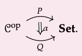
Let C be a small category. A presheaf P on C is a functor P : C\(^{op}\) → Set. To each object c \(\in\) C, we refer to the set P(c) as the set of sections of P over c. To each morphism f : c′ → c, we refer to the function P( f ) : P(c) → P(c′) as the restriction map along f . For any section s \(\in\) P(c), we may denote P( f )(s) \(\in\) P(c′), i.e. its restriction along f, by s|\(_{f}\).

If P and Q are presheaves, a morphism α : P → Q between them is a natural transformation of functors

Example 7.23.

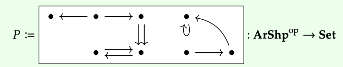
Let ArShp be the category shown below:

The reason we call our category ArShp is that we can imagine of it as an ‘arrow shape.’

A presheaf on ArShp is a functor I : ArShp\(^{op}\) → Set, which is a database instance on ArShp\(^{op}\). Note that ArShp\(^{op}\) is what we called Gr in Section 3.3.5; there we showed that database instances on Gr—i.e. presheaves on ArShp— are just directed graphs, e.g.

Thinking of presheaves on any category C, it often makes sense to imagine the objects of C as shapes of some sort, and the morphisms of C as continuous maps between shapes, just like we did for the arrow shape in Eq. (7.24). In that context, one can think of a presheaf P as a kind of lego construction: P is built out of the shapes in C, connected together using the morphisms in C. In the case where C is the arrow shape, a presheaf is a graph. So this would say that a graph is a sort of lego construction, built out of vertices and arrows connected together using the inclusion of a vertex as the source or target of an arrow. Can you see it?

This statement can be made pretty precise; though we cannot go through it here, the above lego idea is summarized by the formal statement that “the category of presheaves on C is the free colimit completion of C.” Ask a friendly neighborhood category theorist for details.

However one thinks of presheaves in terms of lego assemblies or database instances they’re relatively straightforward. The difference between presheaves and sheaves is that sheaves take into account some sort of ‘covering information.’ The trivial notion of covering is to say that every object covers itself and nothing more; if one uses this trivial covering, presheaves and sheaves are the same thing. In our behavioral context we will need a non-trivial notion of covering, so sheaves and presheaves will be slightly different. Our next goal is to understand sheaves on a topological space.

Topological Spaces

We said in Section 7.3 that, rather than study spaces, we consider spaces as mere ‘sites’ on which things happen. We also said the things that can happen on a space are called sheaves, and always form a type of category called a topos. To define a topos of sheaves, we must start with the site on which they exist.

Sites are very abstract mathematical objects, and we will not make them precise in this book. However, one of the easiest sorts of sites to think about are those coming from topological spaces: every topological space naturally has the structure of a site. We’ve talked about spaces for a while without making them precise; let’s do so now.

Definition 7.25.

Let X be a set, and let \(P(X) = \{U \subseteq X\} denote its set of subsets. A topology on X is a subset Op \(\subseteq\) P(X), elements of which we call open sets,\(^{6}\) satisfying the following conditions:

1. Whole set: the subset X \(\subseteq\) X is open, i.e. X \(\in\) Op.
2. Binary intersections: if U, V \(\in\) Op then (U ∩ V ) \(\in\) Op.
3. Arbitrary unions: if I is a set and if we are given an open set Ui \(\in\) Op for each i, then their union is also open, (\(\bigcup_{i \in I} U_{i}\) \(\in\) Op. We interpret the particular case where I = Ø to mean that the empty set is open: Ø \(\in\) Op.

If \(U = \bigcup_{i \in I} U_{i}\), we say that (Ui)\(_{i \in I}\) covers U.

A pair (X, Op), where X is a set and Op is a topology on X, is called a topological space.

A continuous function between topological spaces (X, Op\(_{X}\) ) and (Y, Op\(_{Y}\)) is a function f :X → Y such that for every U \(\in\) Op\(_{Y}\),the preimage f \(^{−1}\)(U) is in Op\(_{X}\).

At the very end of Section 7.3.1 we mentioned how sheaves differ from presheaves in that they take into account ‘covering information.’ The notion of covering an open set by a union of other open sets was defined in Definition 7.25, and it will come into play when we define sheaves in Definition 7.35.

Example \(\PageIndex{1}\)

The usual topology Op on R2 is based on ‘ε-balls.’ For any ε \(\in\) \(\mathbb{R}\) with ε > 0, and any point p = (x, y) \(\in\) \(\mathbb{R^{2}}\), define the ε-ball centered at p to be:

\(B(p ; \epsilon):=\left\{p^{\prime} \in \mathbb{R}^{2} \mid d\left(p, p^{\prime}\right)<\epsilon\right\}^{7}\)

In other words, B (x, y ; ε) is the set of all points within ε of (x, y).

For an arbitrary subset U \(\subseteq\) \(\mathbb{R^{2}}\),we call it open and put it in Op if,

for every (x, y) \(\in\) U there exists a (small enough) ε > 0 such that B (x, y ; ε) \(\subseteq\) U.

The same idea works if we replace \(\mathbb{R^{2}}\) with any other metric space X (Definition 2.51): it can be considered as a topological space where the open sets are subsets U such that for any p \(\in\) U there is an ε-ball centered at p and contained in U. So every metric space can be considered as a topological space.

Exercise 7.27.

Consider the set \(\mathbb{R}\). It is a metric space with d (x\(_{1}\), x\(_{2}\)) := |x\(_{1}\) − x\(_{2}\) |.

1. What is the 1-dimensional analogue of ε-balls as found in Example 7.26? That is, for each x \(\in\) \(\mathbb{R}\), define B (x, ε).

2. When is an arbitrary subset U \(\subseteq\) \(\mathbb{R}\) called open, in analogy with Example 7.26?

3. Find three open sets U\(_{1}\), U\(_{2}\), and U in \(\mathbb{R}\), such that \(\bigcup_{i \in {1,2}}\) covers U.

4. Find an open set U and a collection \(\bigcup_{i \in I}\) of opens sets where I is infinite, such that \(\bigcup_{i \in I}\) covers U. ♦

Example 7.28.

For any set X, there is a ‘coarsest’ topology, having as few open sets as possible: Op\(_{crse}\) = (Ø, X). There is also a ‘finest’ topology, having as many open sets as possible: Op\(_{fine}\) = P(X). The latter, (X, P(X)) is called the discrete space on the set X.

Exercise 7.29.

1. Verify that for any set X, what we called Op\(_{crse}\) in Example 7.28 really is a topology, i.e. satisfies the conditions of Definition 7.25.

2. Verify also that Op\(_{fine}\) really is a topology.

3. Show that if (X, P(X)) is discrete and (Y, Op\(_{Y}\)) is any topological space, then every function X → Y is continuous. ♦

Example 7.30.

There are four topologies possible on X = {1, 2}. Two are Opcrse and Opfine from Example 7.28. The other two are:

Op\(_{1}\) := {Ø, {1}, X} and Op\(_{2}\) := {Ø, {2}, X}

The two topological spaces ({1, 2}, Op\(_{1}\)) and ({1, 2}, Op\(_{2}\)) are isomorphic; either one can be called the Sierpinski space.

The open sets of a topological space form a preorder. Given a topological space (X, Op), the set Op has the structure of a preorder using the subset relation, (Op, \(\subseteq\)). It is reflexive because U (\subseteq\) U for any U \(\in\) Op, and it is transitive because if U (\subseteq\) V and V (\subseteq\) W then U (\subseteq\) W.

Recall from Section 3.2.3 that we can regard any preorder, and hence Op, as a category: its objects are the open sets U and for any U, V the set of morphisms Op(U, V ) is empty if U (\notsubseteq\) V and it has one element if U (\subseteq\) V.

Exercise 7.31.

Recall the Sierpinski space, say (X, Op\(_{1}\)) from Example 7.30.

1. 1. Write down the Hasse diagram for its preorder of opens.
2. 2. Write down all the covers.

Exercise 7.32.

Given any topological space (X, Op), any subset Y (\subseteq\) X can be given the subspace topology, call it Op\(_{?∩Y}\) .

This topology defines any A (\subseteq\) Y to be open, A \(\in\) Op? ∩Y , if there is an open set B \(\in\) Op such that A = B ∩ Y.

1. Find a B \(\in\) Op that shows that the whole set Y is open, i.e. Y \(\in\) Op\(_{?∩Y}\).

2. Show that Op\(_{?∩Y}\)is a topology in the sense of Definition 7.25.\(^{8}\)

3. Show that the inclusion function Y → X is a continuous function. ♦

Remark 7.33. Suppose (X, Op) is a topological space, and consider the preorder (Op, (\subseteq\)) of open sets. It turns out that (Op, (\subseteq\), X, ∩) is always a quantale in the sense of Definition 2.79. We will not need this fact, but we invite the reader to think about it a bit in Exercise 7.34.

Exercise 7.34.

In Sections 2.3.2 and 2.3.3 we discussed how Bool-categories are pre- orders and Cost-categories are Lawvere metric spaces, and in Section 2.3.4 we imagined interpretations of V-categories for other quantales V.

If (X, Op) is a topological space and V the corresponding quantale as in Remark 7.33, how might we imagine a V-category? ♦

Sheaves on topological spaces

To summarize where we are, a topological space (X, Op) is a set X together with a bunch of subsets we call ‘open’; these open subsets form a preorder and hence category denoted Op. Sheaves on X will be presheaves on Op with a special property, aptly named the ‘sheaf condition.’

Recall the terminology and notation for presheaves: a presheaf on Op is a functor P: Op\(^{op}\) → Set. Thus to every open set U \(\in\) Op we have a set P(U), called the set of sections over U, and to every inclusion of open sets V (\subseteq\) U we have a function P(U) → P(V) called the restriction. If s \(\in\) P(U) is a section over U, we may denote its restriction to V by s|\(_{V}\). Recall that we say a collection of open sets \(\left(U_{i}\right)_{i \in I}\) covers an open set U if U = \(\bigcup_{i \in\ I} U_{i}\).

We are now ready to give the following definition, which comes in several waves: we first define matching families, then gluing, then sheaf condition, then sheaf, and finally the category of sheaves.

Definition 7.35.

Let (X,Op) be a topological space, and let P: Op\(^{op}\) → Set be a presheaf on Op.

Let \(\left(U_{i}\right)_{i \in I}\) be a collection of open sets U\(_{i}\) \(\in\) Op covering U.

A matching family (si)\(_{i \in\I}\) of P-sections over \(\bigcup{i}_{i \in\ I}\) consists of a section si \(\in\) P(Ui) for each i \(\in\) I, such that for every i, j \(\in\) I we have

\(\left.s_{i}\right|_{u_{i} \cap u_{j}}=\left.s_{j}\right|_{U_{i} \cap u_{j}}\)

Given a matching family \(si_{i \in\ I}\) for the cover U = \(\bigcup_{i \in\ I} U_{i}\), we say that s \(\in\) P(U) is a gluing, or glued section, of the matching family if s|\(_{Ui}\) = si holds for all i \(\in\) I. If there exists a unique gluing s \(\in\) P(U) for every matching family \(si_{i \in\ I}\), we say that P satisfies the sheaf condition for the cover U = \(\bigcup_{i \in\ I} U_{i}\). If P satisfies the sheaf condition for every cover, we say that P is a sheaf on (X, Op).

Thus a sheaf is just a presheaf satisfying the sheaf condition for every open cover.

If P and Q are sheaves, then a morphism f : P → Q between these sheaves is just a morphism that is, a natural transformation between their underlying presheaves. We denote by Shv(X, Op) the category of sheaves on X.

The category of sheaves on X is a topos, but we’ll get to that.

Example 7.36.

Here is a funny but very important special case to which the notion of matching family applies. We do not give this example for intuition, but because (to emphasize) it’s an important and easy-to-miss case. Just like the sum of no numbers is 0 and the product of no numbers is 1, the union of no sets is the empty set. Thus if we take U = Ø \(\subseteq\) X and I = Ø, then the empty collection of subsets (one for each i \(\in\) I, of which there are none) covers U. In this case the empty tuple () counts a matching family of sections, and it is the only matching family for the empty cover of the empty set.

In other words, in order for a presheaf P : Op\(^{op}\) → Set to be a sheaf, a necessary (but rarely sufficient) condition is that P(Ø) \(\cong\) {()}, i.e. P(Ø) must be a set with one element.

Extended example: sections of a function. This example is for intuition, and gives a case where the ‘section’ and ‘restriction’ terminology are easy to visualize. Consider the function f : X → Y shown below, where each element of X is sent to the element of Y immediately below it.

For example, f (a\(\_{1}\)) = f (a\(\_{2}\)) = a, f (b\(\_{1}\)) = b, and so on.

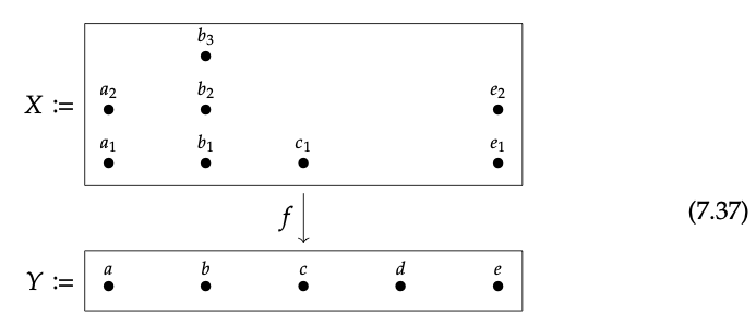
For each point y \(\in\) Y, the preimage set f \(^{−1}\)(y) \(\subseteq\) X above it is often called the fiber over y. Note that different f ’s would arrange the eight elements of X differently over Y: elements of Y would have different fibers.

Exercise 7.38.

Consider the function f : X → Y shown in Eq. (7.37).

1. What is the fiber of f over a?
2. What is the fiber of f over c?
3. What is the fiber of f over d?
4. Gave an example of a function f ′ : X → Y for which every fiber has either one or two elements. ♦

Let’s consider X and Y as discrete topological spaces, so every subset is open, and f is automatically continuous (see Exercise 7.29). We will think of f as an arrangement of X over Y, in terms of fibers as above, and use it to build a sheaf on Y. To do this, we begin by building a presheaf—i.e. a functor Sec f : Op(Y)\(^{op}\) → Set and then we’ll prove it’s a sheaf.

Define the presheaf Sec\(_{f}\) on an arbitrary subset U \(\subseteq\) Y by:

\(\operatorname{Sec}_{f}(U):=\{s: U \rightarrow X \mid(s \text { ; } f)(u)=u \text { for all } u \in U\}\)

One might describe Sec\(_{f}\)(U) as the set of all ways to pick a ‘cross-section’ of the f arrangement over U. That is, an element s \(\in\) Sec\(_{f}\)(U) is a choice of one element per fiber over U. As an example, let’s say U = {a,b}. How many such s ’s are there in Sec\(_{f}\)(U)? To answer this, let’s clip the picture (7.37) and look only at the relevant part:

Looking at the picture (7.39), do you see how we get all cross-sections of f over U?

Exercise 7.40.

Refer to Eq. (7.37).

1. Let V\(_{1}\) = {a, b, c}. Draw all the sections over it, i.e. all elements of Sec\(_{f}\)(V\(_{1}\)), as we did in Eq. (7.39).
2. LetV\(_{2}\) = {a, b, c, d}. Again draw all the sections, Sec\(_{f}\)(V\(_{2}\)).
3. Let V\(_{3}\) = {a, b, d, e}. How many sections (elements of Sec\(_{f}\)(V\(_{3}\))) are there? ♦

By now you should understand the sections of Sec f (U) for various U \(\subseteq\) X. This is Sec\(_{f}\) on objects, so you are half way to understanding Sec\(_{f}\) as a presheaf. That is, as a presheaf, Sec\(_{f}\) also includes a restriction maps for every subset V \(\subseteq\) U.

Luckily, the restriction maps are easy: if V \(\subseteq\) U, say V = {a} and U = {a, b}, then given a section s as in Eq. (7.39), we get a section over V by ‘restricting’ our attention to what s does on {a}.

Exercise 7.42.

1. Write out the sets of sections Sec\(_{f}\)({a,b,c}) and Sec\(_{f}\)({a,c}).
2. Draw lines from the first to the second to indicate the restriction map.

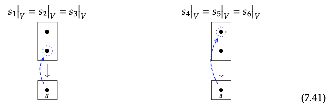
Now we have understood Sec\(_{f}\) as a presheaf; we next explain how to see that it is a sheaf, i.e. that it satisfies the sheaf condition for every cover. To understand the sheaf condition, consider the set U\(_{1}\) = {a, b} and U\(_{2}\) = {b, e}. These cover the set U = {a, b, e} = U\(_{1}\) \(\bigcup\) U\(_{2}\). By Definition 7.35, a matching family for this cover consists of a section over U\(_{1}\) and a section over U\(_{2}\) that agree on the overlap set, U\(_{1}\) ∩ U\(_{2}\) = {b}.

So consider s\(_{1}\) \(\in\) Sec f (U\(_{1}\)) and s\(_{2}\) \(\in\) Sec\(_{f}\)(U\(_{2}\)) shown below.

Since sections g\(_{1}\) and g\(_{2}\) agree on the overlap they both send b to b\(_{2}\) the two sections 122 shown in Eq. (7.43) can be glued to form a single section over U = {a, b, e}:

Exercise 7.44.

Again let U\(_{1}\) = {a, b} and U\(_{2}\) = {b, e}, so the overlap is U\(_{1}\) ∩ U\(_{2}\) = {b}.

1. Find a section s\(_{1}\) \(\in\) Sec\(_{f}\) (U\(_{1}\)) and a section s\(_{2}\) \(\in\) Sec\(_{f}\)(U\(_{2}\)) that do not agree on the overlap.
2. For your answer (s\(_{1}\), s\(_{2}\)) in part 1, can you find a section s \(\in\) Sec\(_{f}\) (U\(_{1}\) \(\bigcup\) U\(_{2}\)) such that s|\(_{U_{1}}\) = s\(_{1}\) and s|(_{U_{2}}\) = s\(_{2}\)?
3. Find a section h\(_{1}\) \(\in\) Sec\(_{f}\) (U\(_{1}\)) and a section h\(_{2}\) \(\in\) Sec\(_{f}\)(U\(_{2}\)) that do agree on the overlap, but which are different than our choice in Eq. (7.43).
4. Can you find a section h \(\in\) Sec\(_{f}\)(U\(_{1}\) \(\bigcup\) U\(_{2}\)) such that h|\(_{U_{1}}\) = h\(_{1}\) and h |\(_{U_{2}}\) = h\(_{2}\)? ♦

Other examples of sheaves. The extended example above generalizes to any contin- uous function f : X → Y between topological spaces.

Example 7.45.

Let f : (X, Op\(_{X}\)) → (Y, Op\(_{Y}\)) be a continuous function. Consider the op functor \(\mathrm{Sec}_{f}: \mathrm{Op}_{Y}^{\mathrm{op}} \rightarrow \text { Set }\) → Set given by

Sec\(_{f}\)(U) := {g: U → X | g is continuous and (g ; f )(u) = u for all u \(\in\) U},

The morphisms of Op\(_{Y}\) are inclusions V \(\subseteq\) U. Given g : U → X and V \(\subseteq\) U, what we call the restriction of g to V is the usual thing we mean by restriction, the same as it was in Eq.(7.41). One can again check that Sec\(_{f}\) is a sheaf.

Example 7.46.

A nice example of a sheaf on a space M is that of vector fields on M. If you calculate the wind velocity at every point on Earth, you will have what’s called a vector field on Earth. If you know the wind velocity at every point in Afghanistan and I know the wind velocity at every point in Pakistan, and our calculations agree around the border, then we can glue our information together to get the wind velocity over the union of the two countries. All possible wind velocity fields over all possible open sets of the Earth’s surface together form the sheaf of vector fields.

Let’s say this a bit more formally. A manifold M you can just imagine a sphere such as the Earth’s surface always has something called a tangent bundle. It is a space TM whose points are pairs (m, v), where m \(\in\) M is a point in the manifold and v is a tangent vector emanating from it. Here’s a picture of one tangent plane all the tangent vectors emanating from some fixed point on a sphere:

The tangent bundle TM includes the whole tangent plane shown above including the three vectors drawn on it—as well as the tangent plane at every other point on the sphere.

The tangent bundle TM on a manifold M comes with a continuous map π: TM → M back down to the manifold, sending (m, v) \(\longmapsto\) m. One might say that π “forgets the tangent vector and just remembers the point it emanated from.” By Example 7.45, π defines a sheaf Sec\(_{pi}\). It could be called the sheaf of ‘tangent vector sections on M’, but its usual name is the sheaf of vector fields on M. This is what we were describing when we spoke of the sheaf of wind velocities on Earth, above. Given an open subset U ⊆ M, an element v \(\in\) Sec\(_{pi}\)(U) is called a vector field over U because it continuously assigns a tangent vector v(u) to each point u \(\in\) U. The tangent vector at u tells us the velocity of the wind at that point.

Here’s a fun digression: in the case of a spherical manifold M like the Earth, it’s possible to prove that for every open set U, as long as U \(\neq\) M, there is a vector field v \(\in\) Sec\(_{pi}\)(U) that is never 0: the wind could be blowing throughout U. However, a theorem of Poincaré says that if you look at the whole sphere, there is guaranteed to be a point m \(\in\) M at which the wind is not blowing at all. It’s like the eye of a hurricane or perhaps a cowlick. A cowlick in someone’s hair occurs when the hair has no direction to go, so it sticks up! Hair sticking up would not count as a tangent vector: tangent vectors must start out lying flat along the head. Poincaré proved that if your head was covered completely with inch-long hair, there would be at least one cowlick. This difference between local sections (over arbitrary U \(\subseteq\) X) and global sections (over X) namely that hair can be well combed whenever U \(\neq\) X but cannot be well combed when U = X can be thought of as a generative effect, and can be measured by cohomology (see Section 1.5).

Exercise 7.47.

If M is a sphere as in Example 7.46, we know from Definition 7.35 that we can consider the category Shv(M) of sheaves on M; in fact, such categories are toposes and these are what we’re getting to.

But are the sheaves on M the vector fields? That is, is there a one-to-one correspondence between sheaves on M and vector sheaves on M and vector fields on M ? If so, why? If not, how are sheaves on M and vector fields on M related? ♦

Example 7.48.

For every topological space (X, Op), we have the topos of sheaves on it. The topos of sets, which one can regard as the story of set theory, is the category of sheaves on the one-point space {∗}. In topos theory, we see the category of sets an huge, amazing, and rich category as corresponding to a single point. Imagine how much more complex arbitrary toposes are, when they can take place on much more interesting topological spaces (and in fact even more general ‘sites’).

Exercise 7.49.

Consider the Sierpinski space ({1,2}, Op\(_{1}\)) from Example 7.30.

1. What is the category Op for this space? (You may have already figured this out in Exercise 7.31; if not, do so now.)
2. What does a presheaf on Op consist of?
3. What is the sheaf condition for Op?
4. How do we identify a sheaf on Op with a function? ♦