1.5: Quadratics
- Page ID
- 71043
\( \newcommand{\vecs}[1]{\overset { \scriptstyle \rightharpoonup} {\mathbf{#1}} } \)
\( \newcommand{\vecd}[1]{\overset{-\!-\!\rightharpoonup}{\vphantom{a}\smash {#1}}} \)
\( \newcommand{\dsum}{\displaystyle\sum\limits} \)
\( \newcommand{\dint}{\displaystyle\int\limits} \)
\( \newcommand{\dlim}{\displaystyle\lim\limits} \)
\( \newcommand{\id}{\mathrm{id}}\) \( \newcommand{\Span}{\mathrm{span}}\)
( \newcommand{\kernel}{\mathrm{null}\,}\) \( \newcommand{\range}{\mathrm{range}\,}\)
\( \newcommand{\RealPart}{\mathrm{Re}}\) \( \newcommand{\ImaginaryPart}{\mathrm{Im}}\)
\( \newcommand{\Argument}{\mathrm{Arg}}\) \( \newcommand{\norm}[1]{\| #1 \|}\)
\( \newcommand{\inner}[2]{\langle #1, #2 \rangle}\)
\( \newcommand{\Span}{\mathrm{span}}\)
\( \newcommand{\id}{\mathrm{id}}\)
\( \newcommand{\Span}{\mathrm{span}}\)
\( \newcommand{\kernel}{\mathrm{null}\,}\)
\( \newcommand{\range}{\mathrm{range}\,}\)
\( \newcommand{\RealPart}{\mathrm{Re}}\)
\( \newcommand{\ImaginaryPart}{\mathrm{Im}}\)
\( \newcommand{\Argument}{\mathrm{Arg}}\)
\( \newcommand{\norm}[1]{\| #1 \|}\)
\( \newcommand{\inner}[2]{\langle #1, #2 \rangle}\)
\( \newcommand{\Span}{\mathrm{span}}\) \( \newcommand{\AA}{\unicode[.8,0]{x212B}}\)
\( \newcommand{\vectorA}[1]{\vec{#1}} % arrow\)
\( \newcommand{\vectorAt}[1]{\vec{\text{#1}}} % arrow\)
\( \newcommand{\vectorB}[1]{\overset { \scriptstyle \rightharpoonup} {\mathbf{#1}} } \)
\( \newcommand{\vectorC}[1]{\textbf{#1}} \)
\( \newcommand{\vectorD}[1]{\overrightarrow{#1}} \)
\( \newcommand{\vectorDt}[1]{\overrightarrow{\text{#1}}} \)
\( \newcommand{\vectE}[1]{\overset{-\!-\!\rightharpoonup}{\vphantom{a}\smash{\mathbf {#1}}}} \)
\( \newcommand{\vecs}[1]{\overset { \scriptstyle \rightharpoonup} {\mathbf{#1}} } \)
\(\newcommand{\longvect}{\overrightarrow}\)
\( \newcommand{\vecd}[1]{\overset{-\!-\!\rightharpoonup}{\vphantom{a}\smash {#1}}} \)
\(\newcommand{\avec}{\mathbf a}\) \(\newcommand{\bvec}{\mathbf b}\) \(\newcommand{\cvec}{\mathbf c}\) \(\newcommand{\dvec}{\mathbf d}\) \(\newcommand{\dtil}{\widetilde{\mathbf d}}\) \(\newcommand{\evec}{\mathbf e}\) \(\newcommand{\fvec}{\mathbf f}\) \(\newcommand{\nvec}{\mathbf n}\) \(\newcommand{\pvec}{\mathbf p}\) \(\newcommand{\qvec}{\mathbf q}\) \(\newcommand{\svec}{\mathbf s}\) \(\newcommand{\tvec}{\mathbf t}\) \(\newcommand{\uvec}{\mathbf u}\) \(\newcommand{\vvec}{\mathbf v}\) \(\newcommand{\wvec}{\mathbf w}\) \(\newcommand{\xvec}{\mathbf x}\) \(\newcommand{\yvec}{\mathbf y}\) \(\newcommand{\zvec}{\mathbf z}\) \(\newcommand{\rvec}{\mathbf r}\) \(\newcommand{\mvec}{\mathbf m}\) \(\newcommand{\zerovec}{\mathbf 0}\) \(\newcommand{\onevec}{\mathbf 1}\) \(\newcommand{\real}{\mathbb R}\) \(\newcommand{\twovec}[2]{\left[\begin{array}{r}#1 \\ #2 \end{array}\right]}\) \(\newcommand{\ctwovec}[2]{\left[\begin{array}{c}#1 \\ #2 \end{array}\right]}\) \(\newcommand{\threevec}[3]{\left[\begin{array}{r}#1 \\ #2 \\ #3 \end{array}\right]}\) \(\newcommand{\cthreevec}[3]{\left[\begin{array}{c}#1 \\ #2 \\ #3 \end{array}\right]}\) \(\newcommand{\fourvec}[4]{\left[\begin{array}{r}#1 \\ #2 \\ #3 \\ #4 \end{array}\right]}\) \(\newcommand{\cfourvec}[4]{\left[\begin{array}{c}#1 \\ #2 \\ #3 \\ #4 \end{array}\right]}\) \(\newcommand{\fivevec}[5]{\left[\begin{array}{r}#1 \\ #2 \\ #3 \\ #4 \\ #5 \\ \end{array}\right]}\) \(\newcommand{\cfivevec}[5]{\left[\begin{array}{c}#1 \\ #2 \\ #3 \\ #4 \\ #5 \\ \end{array}\right]}\) \(\newcommand{\mattwo}[4]{\left[\begin{array}{rr}#1 \amp #2 \\ #3 \amp #4 \\ \end{array}\right]}\) \(\newcommand{\laspan}[1]{\text{Span}\{#1\}}\) \(\newcommand{\bcal}{\cal B}\) \(\newcommand{\ccal}{\cal C}\) \(\newcommand{\scal}{\cal S}\) \(\newcommand{\wcal}{\cal W}\) \(\newcommand{\ecal}{\cal E}\) \(\newcommand{\coords}[2]{\left\{#1\right\}_{#2}}\) \(\newcommand{\gray}[1]{\color{gray}{#1}}\) \(\newcommand{\lgray}[1]{\color{lightgray}{#1}}\) \(\newcommand{\rank}{\operatorname{rank}}\) \(\newcommand{\row}{\text{Row}}\) \(\newcommand{\col}{\text{Col}}\) \(\renewcommand{\row}{\text{Row}}\) \(\newcommand{\nul}{\text{Nul}}\) \(\newcommand{\var}{\text{Var}}\) \(\newcommand{\corr}{\text{corr}}\) \(\newcommand{\len}[1]{\left|#1\right|}\) \(\newcommand{\bbar}{\overline{\bvec}}\) \(\newcommand{\bhat}{\widehat{\bvec}}\) \(\newcommand{\bperp}{\bvec^\perp}\) \(\newcommand{\xhat}{\widehat{\xvec}}\) \(\newcommand{\vhat}{\widehat{\vvec}}\) \(\newcommand{\uhat}{\widehat{\uvec}}\) \(\newcommand{\what}{\widehat{\wvec}}\) \(\newcommand{\Sighat}{\widehat{\Sigma}}\) \(\newcommand{\lt}{<}\) \(\newcommand{\gt}{>}\) \(\newcommand{\amp}{&}\) \(\definecolor{fillinmathshade}{gray}{0.9}\)Quadratics are transformations of the function \( f(x)=x^2 \). Quadratics commonly arise from problems involving area and projectile motion, providing some interesting applications.
A backyard farmer wants to enclose a rectangular space for a new garden. She has purchased 80 feet of wire fencing to enclose three sides, and will put the fourth side against the backyard fence. Find a formula for the area enclosed by the fence if the sides of fencing perpendicular to the existing fence have length \(L\).
Solution
In a scenario like this involving geometry, it is often helpful to draw a picture. It might also be helpful to introduce a temporary variable, \(W\), to represent the side of fencing parallel to the fourth side or backyard fence.
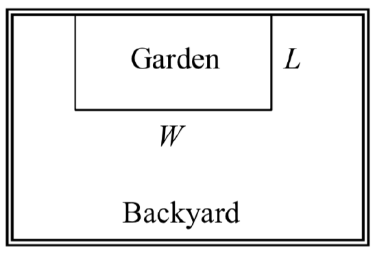
Since we know we only have 80 feet of fence available, we know that \( L+W+L=80 \), or more simply, \( 2L+W=80 \). This allows us to represent the width, \(W\), in terms of \(L\): \( W=80-2L \)
Now we are ready to write an equation for the area the fence encloses. We know the area of a rectangle is length multiplied by width, so \( A=LW=L(80-2l) \), so \[ A(L)=80L-2L^2. \nonumber \] This formula represents the area of the fence in terms of the variable length \(L\).
A local newspaper currently has 84,000 subscribers, at a quarterly charge of $30. Market research has suggested that if they raised the price to $32, they would lose 5,000 subscribers. Assuming that subscriptions are linearly related to the price, create an equation to model their revenue as a function of the quarterly charge.
Solution
Revenue is the amount of money a company brings in. In this case, the revenue can be found by multiplying the charge per subscription times the number of subscribers. We can introduce variables, \(C\) for charge per subscription and \(S\) for the number subscribers, giving us the equation:
Revenue = \(C S\)
Since the number of subscribers changes with the price, we need to find a relationship between the variables.
We know that currently \(S = 84,000\) and \(C = 30\), and that if they raise the price to $32 they would lose 5,000 subscribers, giving a second pair of values, \(S = 79,000\) and \(C = 32\). From this we can find a linear equation relating the two quantities. Treating \(C\) as the input and \(S\) as the output, the equation will have form \(S = mC + b\). The slope will be
\[m = \dfrac{79,000 - 84,000}{32-30} = \dfrac{-5,000}{2} = -2,500\nonumber \]This tells us the paper will lose 2,500 subscribers for each dollar they raise the price. We can then solve for the vertical intercept.
\[S = -2500C + b\nonumber \]
Plug in the point \(S = 84,000\) and \(C = 30\)
\[84000 = -2500(30) + b\nonumber \]
Solve for \(b\)
\[b = 159,000\nonumber \]
This gives us the linear equation \(S = -2,500C + 159,000\) relating cost and subscribers. Note this is a demand equation where \(C\) is the price and \(S\) is the quantity demanded. We now return to our revenue equation.
Revenue = \(C S\)
Substituting the equation for \(S\) from above:
Revenue = \(C \left(-2,500C + 159,000\right)\)
Expanding
Revenue = \(-2,500C^2 + 159,000C\)
We now have a quadratic equation for revenue as a function of the subscription charge. Later in the course we will use equations like this to determine the price to charge to maximize revenue.
The standard form of a quadratic function is \( f(x)=ax^2+bx+c \).
The transformation form of a quadratic function is \( f(x)=a(x-h)^2+k \).
The vertex of the quadratic function is located at \((h, k)\), where \(h\) and \(k\) are the numbers in the transformation form of the function. Because the vertex appears in the transformation form, it is often called the vertex form.
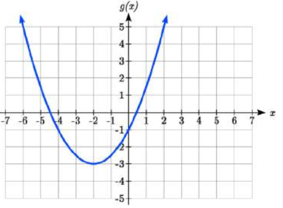
Write an equation for the quadratic graphed below as a transformation of \( f(x)=x^2 \).
Solution
We can see the graph is the basic quadratic shifted to the left 2 and down 3, putting the vertex at \((-2, -3)\), giving a formula in the form \( g(x)=a(x+2)^2-3 \). By plugging in a point that falls on the grid, such as \((0,-1)\), we can solve for the stretch factor: \[\begin{align*} -1 & = a(0+2)^2-3 \\ 2 & = 4a \\ a & = \frac{1}{2} \end{align*}\nonumber \]
The equation for this formula is \[ g(x)=\frac{1}{2}(x+2)^2-3 \nonumber \]
Short run Behavior: Intercepts
As with any function, we can find the vertical intercepts of a quadratic by evaluating the function at an input of zero, and we can find the horizontal intercepts by solving for when the output will be zero. Notice that depending upon the location of the graph, we might have zero, one, or two horizontal intercepts.
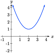
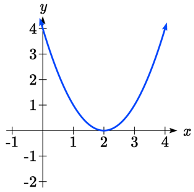
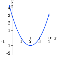
Notice that in the standard form of a quadratic, the constant term \(c\) reveals the vertical intercept of the graph, since \( f(0)=a(0)^2+b(0)+c=c \).
Find the vertical and horizontal intercepts of the quadratic \( f(x)=3x^2+5x-2 \).
Solution
We can find the vertical intercept by evaluating the function at an input of zero: \[f(0)=3(0)^2+5(0)-2=-2\nonumber \] So the vertical intercept is at (0,-2)
For the horizontal intercepts, we solve for when the output will be zero: \[0=3x^2+5x-2.\nonumber \] In this case, the quadratic can be factored easily, providing the simplest method for solution.: \[0=(3x-1)(x+2),\nonumber \] so either \[ \begin{align*} 0 & = 3x-1\\ x & = \frac{1}{3} \end{align*} \nonumber \] or \[ \begin{align*} 0 & = x+2\\ x & = -2 \end{align*} \nonumber \] So the Horizontal intercepts are at \( \left(\frac{1}{3},0\right) \) and \((-2,0)\).
When a quadratic is not factorable or is hard to factor, we can turn to the quadratic formula.
For a quadratic function given in standard form \( f(x)=ax^2+bx+c \), the quadratic formula gives the horizontal intercepts of the graph of this function:\[ x=\frac{-b\pm \sqrt{b^2-4ac}}{2a} \nonumber \]
A ball is thrown upwards from the top of a 40 foot high building at a speed of 80 feet per second. The ball’s height above ground can be modeled by the equation \[ H(t)=-16t^2+80t+40 .\nonumber \] When does the ball hit the ground?
Solution
To find when the ball hits the ground, we need to determine when the height is zero, i.e., when \(H(t) = 0\). While we could do this using the transformation form of the quadratic, we can also use the quadratic formula: \[ t=\frac{-80\pm \sqrt{80^2-4(-16)(40)}}{2(-16)}=\frac{-80\pm\sqrt{8960}}{-32} \nonumber \]
Since the square root does not simplify nicely, we can use a calculator to approximate the values of the solutions:\[ t=\frac{-80-\sqrt{8960}}{-32}\approx 5.458 \quad\text{or}\quad t=\frac{-80+\sqrt{8960}}{-32}\approx -0.458 \nonumber \]
The second answer is outside the reasonable domain of our model, so we conclude the ball will hit the ground after about 5.458 seconds.
The supply for a certain product can be modeled by \(p = 3q^2\) and the demand can be modeled by \(p = 1620 - 2q^2\), where \(p\) is the price in dollars, and \(q\) is the quantity in thousands of items. Find the equilibrium price and quantity.
Solution
Recall that the equilibrium price and quantity is found by finding where the supply and demand curve intersect. We can find that by setting the equations equal: \[3q^2 = 1620 - 2q^2\nonumber\]
Add \(2q^2\) to both sides: \(5q^2 = 1620\)
Divide by 5 on both sides: \(q^2 = 324\)
Take the square root of both sides: \[q = \pm \sqrt{324} = \pm 18 \nonumber\]
Since it doesn’t make sense to talk about negative quantities, the equilibrium quantity is \(q = 18\). To find the equilibrium price, we evaluate either function at the equilibrium quantity. \[p = 3(18)^2 = 972\nonumber\]
The equilibrium is 18 thousand items, at a price of $972.


