2.6: Derivatives of Inverse Functions

Learning Objectives

In this section, we strive to understand the ideas generated by the following important questions:

• What is the derivative of the natural logarithm function?
• What are the derivatives of the inverse trigonometric functions \(arcsin(x)\) and \(arctan(x)\)?
• If \(g\) is the inverse of a differentiable function \(f\), how is \(g'\) computed in terms of \(f\), \(f'\), and \(g\)?

Much of mathematics centers on the notion of function. Indeed, throughout our study of calculus, we are investigating the behavior of functions, often doing so with particular emphasis on how fast the output of the function changes in response to changes in the input. Because each function represents a process, a natural question to ask is whether or not the particular process can be reversed. That is, if we know the output that results from the function, can we determine the input that led to it? Connected to this question, we now also ask: if we know how fast a particular process is changing, can we determine how fast the inverse process is changing?

As we have noted, one of the most important functions in all of mathematics is the natural exponential function \(f (x) = e^x\). Because the natural logarithm, \(g(x) = \ln (x)\), is the inverse of the natural exponential function, the natural logarithm is similarly important. One of our goals in this section is to learn how to differentiate the logarithm function, and thus expand our library of basic functions with known derivative formulas. First, we investigate a more familiar setting to refresh some of the basic concepts surrounding functions and their inverses.

Preview Activity \(\PageIndex{1}\)

The equation \(y = \dfrac{5}{9} (x - 32)\) relates a temperature given in \(x\) degrees Fahrenheit to the corresponding temperature \(y\) measured in degrees Celsius.

1. Solve the equation y = 5 9 (x - 32) for x to write x (Fahrenheit temperature) in terms of y (Celcius temperature).
2. Let C(x) = 5 9 (x - 32) be the function that takes a Fahrenheit temperature as input and produces the Celcius temperature as output. In addition, let F(y) be the function that converts a temperature given in y degrees Celcius to the temperature F(y) measured in degrees Fahrenheit. Use your work in (a) to write a formula for F(y). 130
3. Next consider the new function defined by p(x) = F(C(x)). Use the formulas for F and C to determine an expression for p(x) and simplify this expression as much as possible. What do you observe?
4. Now, let r(y) = C(F(y)). Use the formulas for F and C to determine an expression for r(y) and simplify this expression as much as possible. What do you observe?
5. What is the value of C 0 (x)? of F 0 (y)? How do these values appear to be related? ./

Basic Facts about Inverse Functions

A function f : A → B is a rule that associates each element in the set A to one and only one element in the set B. We call A the domain of f and B the codomain of f . If there exists a function g : B → A such that g( f (a)) = a for every possible choice of a in the set A and f (g(b)) = b for every b in the set B, then we say that g is the inverse of f . We often use the notation f -1 (read “f -inverse”) to denote the inverse of f . Perhaps the most essential thing to observe about the inverse function is that it undoes the work of f . Indeed, if y = f (x), then

\[f -1 (y) = f -1 ( f (x)) = x,\]

and this leads us to another key observation: writing y = f (x) and x = f -1 (y) say the exact same thing. The only difference between the two equations is one of perspective – one is solved for x, while the other is solved for y. Here we briefly remind ourselves of some key facts about inverse functions. For a function f : A → B,

• f has an inverse if and only if f is one-to-one8 and onto9 ;
• provided f -1 exists, the domain of f -1 is the codomain of f , and the codomain of f -1 is the domain of f ;
• f -1 ( f (x)) = x for every x in the domain of f and f ( f -1 (y)) = y for every y in the codomain of f ;
• y = f (x) if and only if x = f -1 (y).

The last stated fact reveals a special relationship between the graphs of f and f -1 . In particular, if we consider y = f (x) and a point (x, y) that lies on the graph of f , then it is also true that x = f -1 (y), which means that the point (y, x) lies on the graph of f -1 .

Note

• A function \(f\) is one-to-one provided that no two distinct inputs lead to the same output.
• A function \(f\) is onto provided that every possible element of the codomain can be realized as an output of the function for some choice of input from the domain.

This shows us that the graphs of f and f -1 are the reflections of one another across the line y = x, since reflecting across y = x is precisely the geometric action that swaps the coordinates in an ordered pair. In Figure 2.8, we see this exemplified for the function y = f (x) = 2 x and its inverse, with the points (-1, 1 2 ) and ( 1 2 , -1) highlighting the reflection of the curves across y = x.

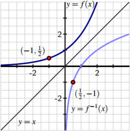
Figure 2.8: A graph of a function y = f (x) along with its inverse, y = f -1 (x).

To close our review of important facts about inverses, we recall that the natural exponential function y = f (x) = e x has an inverse function, and its inverse is the natural logarithm, x = f -1 (y) = \ln (y). Indeed, writing y = e x is interchangeable with x = \ln (y), plus \ln (e x ) = x for every real number x and e \ln (y) = y for every positive real number y.

The Derivative of the Natural Logarithm Function

In what follows, we determine a formula for the derivative of \(g(x) = \ln (x)\). To do so, we take advantage of the fact that we know the derivative of the natural exponential function, which is the inverse of g. In particular, we know that writing \(g(x) = \ln (x)\) is equivalent to writing \(e^{g(x)} = x\). Now we differentiate both sides of this most recent equation. In particular, we observe that

\[\dfrac{d}{dx} \left[ e^{g(x)} \right] = \dfrac{d}{dx} [x]. \label{eqLog}\]

The righthand side of Equaton \ref{eqLog} is simply 1; applying the chain rule to the left side, we find that

\[e^{g(x)} g'(x) = 1 \label{eq10}\]

Since our goal is to determine \(g'(x)\), we solve Equation \ref{eq10} for \(g'(x)\), so

\[g' (x) = 1 e^{g(x)}. \label{eq11}\]

Finally, we recall that since

\[g(x) = \ln (x)\]

which when substituted into Equation \ref{eq11} results in

\[e^{g(x)} = e^{\ln (x)} = x\]

and thus

\[g' (x) = \dfrac{1}{x}.\]

Natural Logarithm

For all positive real numbers \(x\),

\[\dfrac{d}{dx} [\ln (x)] = \dfrac{1}{x}.\]

This rule for the natural logarithm function now joins our list of other basic derivative rules that we have already established. There are two particularly interesting things to note about the fact that d dx [\ln (x)] = 1 x . One is that this rule is restricted to only apply to positive values of x, as these are the only values for which the original function is defined. The other is that for the first time in our work, differentiating a basic function of a particular type has led to a function of a very different nature: the derivative of the natural logarithm is not another logarithm, nor even an exponential function, but rather a rational one. Derivatives of logarithms may now be computed in concert with all of the rules known to date. For instance, if f(t) = \ln (t 2 + 1), then by the chain rule, f 0 (t) = 1 t 2+1 · 2t.

Activity \(\PageIndex{1}\):

For each function given below, find its derivative.

1. h(x) = x 2 \ln (x)
2. p(t) = \ln (t) e t + 1
3. s(y) = \ln (cos(y) + 2)
4. z(x) = tan(\ln (x))
5. m(z) = \ln (\ln (z)) C

In addition to the important rule we have derived for the derivative of the natural log functions, there are additional interesting connections to note between the graphs of f (x) = e x and f -1 (x) = \ln (x).

In Figure 2.9, we are reminded that since the natural exponential function has the property that its derivative is itself, the slope of the tangent to y = e x is equal to the height of the curve at that point. For instance, at the point A = (\ln (0.5), 0.5), the slope of the tangent line is mA = 0.5, and at B = (\ln (5), 5), the tangent line’s slope is mB = 5. At the corresponding points A 0 and B 0 on the graph of the natural logarithm function (which come from reflecting across the line y = x), we know that the slope of the tangent line is the reciprocal of the x-coordinate of the point (since d dx [\ln (x)] = 1 x ). Thus, with A 0 = (0.5, \ln (0.5)), we have mA0 = 1 0.5 = 2, and at B 0 = (5, \ln (5)), mB0 = 1 5 .

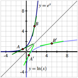
Figure 2.9: A graph of the function y = e x along with its inverse, y = \ln (x), where both functions are viewed using the input variable x.

In particular, we observe that mA0 = 1 mA and mB0 = 1 mB . This is not a coincidence, but in fact holds for any curve y = f (x) and its inverse, provided the inverse exists. One rationale for why this is the case is due to the reflection across y = x: in so doing, we essentially change the roles of x and y, thus reversing the rise and run, which leads to the slope of the inverse function at the reflected point being the reciprocal of the slope of the original function. At the close of this section, we will also look at how the chain rule provides us with an algebraic formulation of this general phenomenon.

Inverse Trigonometric Functions and their Derivatives

Trigonometric functions are periodic, so they fail to be one-to-one, and thus do not have inverses. However, if we restrict the domain of each trigonometric function, we can force the function to be one-to-one. For instance, consider the sine function on the domain [- π 2 , π 2 ].

Because no output of the sine function is repeated on this interval, the function is one-to-one and thus has an inverse. In particular, if we view f (x) = sin(x) as having domain [- π 2 , π 2 ] and codomain [-1, 1], then there exists an inverse function f -1 such that

\[f -1 : [-1, 1] → [- π 2 , π 2 ]. \]

We call f -1 the arcsine (or inverse sine) function and write f -1 (y) = arcsin(y). It is especially important to remember that writing

\[y = \sin(x) and x = arcsin(y) \]

say the exact same thing. We often read “the arcsine of y” as “the angle whose sine is y.”

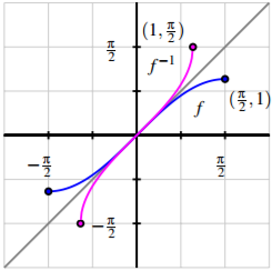
Figure 2.10: A graph of f (x) = sin(x) (in blue), restricted to the domain [- π 2 , π 2 ], along with its inverse, f -1 (x) = arcsin(x) (in magenta).

For example, we say that π 6 is the angle whose sine is 1 2 , which can be written more concisely as arcsin( 1 2 ) = π 6 , which is equivalent to writing sin( π 6 ) = 1 2 . Next, we determine the derivative of the arcsine function. Letting h(x) = arcsin(x), our goal is to find h 0 (x). Since \(h(x)\) is the angle whose sine is \(x\), it is equivalent to write

\[\sin(h(x)) = x.\]

Differentiating both sides of the previous equation, we have

\[d dx [sin(h(x))] = d dx [x], \]

and by the fact that the righthand side is simply 1 and by the chain rule applied to the left side,

\[cos(h(x))h 0 (x) = 1.\]

Solving for h 0 (x), it follows that h 0 (x) = 1 cos(h(x)). Finally, we recall that h(x) = arcsin(x), so the denominator of h 0 (x) is the function cos(arcsin(x)), or in other words, “the cosine of the angle whose sine is x.” A bit of right triangle trigonometry allows us to simplify this expression considerably. Let’s say that θ = arcsin(x), so that θ is the angle whose sine is x. From this, it follows that we can picture θ as an angle in a right triangle with hypotenuse 1 and a vertical leg of length x, as shown in Figure 2.11. The horizontal leg must be √ 1 - x 2, by the Pythagorean Theorem. Now, note particularly that θ = arcsin(x) since sin(θ) = x, and recall that we want to know a different expression for cos(arcsin(x)).

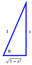
Figure 2.11: The right triangle that corresponds to the angle θ = arcsin(x).

From the figure, cos(arcsin(x)) = cos(θ) = √ 1 - x 2. Thus, returning to our earlier work where we established that if

\[h(x) = arcsin(x),\]

then

\[h' (x) = \dfrac{1}{cos(arcsin(x))}\]

we have now shown that

\[h ' (x) = \dfrac{1}{\sqrt{1 - x^2}}.\]

Inverse sine

For all real numbers \(x\) such that \(-1 < x < 1\), \[\dfrac{d}{dx} [\text{arcsin}(x)] = \dfrac{1}{\sqrt{1 - x^ 2}}.\]

Activity \(\PageIndex{2}\):

The following prompts in this activity will lead you to develop the derivative of the inverse tangent function.

1. Let r(x) = arctan(x). Use the relationship between the arctangent and tangent functions to rewrite this equation using only the tangent function.
2. Differentiate both sides of the equation you found in (a). Solve the resulting equation for r 0 (x), writing r 0 (x) as simply as possible in terms of a trigonometric function evaluated at r(x).
3. Recall that r(x) = arctan(x). Update your expression for r 0 (x) so that it only involves trigonometric functions and the independent variable x.
4. Introduce a right triangle with angle θ so that θ = arctan(x). What are the three sides of the triangle?
5. In terms of only x and 1, what is the value of cos(arctan(x))? 136
6. Use the results of your work above to find an expression involving only 1 and x for r 0 (x).

While derivatives for other inverse trigonometric functions can be established similarly, we primarily limit ourselves to the arcsine and arctangent functions. With these rules added to our library of derivatives of basic functions, we can differentiate even more functions using derivative shortcuts. In Activity 2.18, we see each of these rules at work.

Activity \(\PageIndex{3}\):

Determine the derivative of each of the following functions.

1. f (x) = x 3 arctan(x) + e x \ln (x)
2. p(t) = 2 t arcsin(t)
3. h(z) = (arcsin(5z) + arctan(4 - z))27
4. s(y) = cot(arctan(y))
5. m(v) = \ln (sin2 (v) + 1)
6. g(w) = arctan \ln (w) 1 + w2 !

The link between the derivative of a function and the derivative of its inverse In Figure 2.9, we saw an interesting relationship between the slopes of tangent lines to the natural exponential and natural logarithm functions at points that corresponded to reflection across the line y = x. In particular, we observed that for a point such as (\ln (2), 2) on the graph of f (x) = e x , the slope of the tangent line at this point is f 0 (\ln (2)) = 2, while at the corresponding point (2, \ln (2)) on the graph of f -1 (x) = \ln (x), the slope of the tangent line at this point is ( f -1 ) 0 (2) = 1 2 , which is the reciprocal of f 0 (\ln (2)). That the two corresponding tangent lines having slopes that are reciprocals of one another is not a coincidence. If we consider the general setting of a differentiable function f with differentiable inverse g such that y = f (x) if and only if x = g(y), then we know that f (g(x)) = x for every x in the domain of f -1 . Differentiating both sides of this equation with respect to x, we have d dx [ f (g(x))] = d dx [x], and by the chain rule, f 0 (g(x))g 0 (x) = 1. 137 Solving for g 0 (x), we have g 0 (x) = 1 f 0 (g(x)) . Here we see that the slope of the tangent line to the inverse function g at the point (x, g(x)) is precisely the reciprocal of the slope of the tangent line to the original function f at the point (g(x), f (g(x))) = (g(x), x).

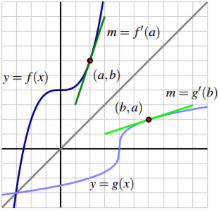
Figure 2.12: A graph of function y = f (x) along with its inverse, y = g(x) = f -1 (x). Observe that the slopes of the two tangent lines are reciprocals of one another.

To see this more clearly, consider the graph of the function y = f (x) shown in Figure 2.12, along with its inverse y = g(x). Given a point (a, b) that lies on the graph of f , we know that (b, a) lies on the graph of g; said differently, f (a) = b and g(b) = a. Now, applying the rule that g 0 (x) = 1/ f 0 (g(x)) to the value x = b, we have g 0 (b) = 1 f 0 (g(b)) = 1 f 0 (a) , which is precisely what we see in the figure: the slope of the tangent line to g at (b, a) is the reciprocal of the slope of the tangent line to f at (a, b), since these two lines are reflections of one another across the line y = x. Derivative of an inverse function: Suppose that f is a differentiable function with inverse g and that (a, b) is a point that lies on the graph of f at which f 0 (a) , 0. Then g 0 (b) = 1 f 0 (a) . More generally, for any x in the domain of g 0 , we have g 0 (x) = 1/ f 0 (g(x)). The rules we derived for \ln (x), arcsin(x), and arctan(x) are all just specific examples of this general property of the derivative of an inverse function. For example, with 138 g(x) = \ln (x) and f (x) = e x , it follows that g 0 (x) = 1 f 0 (g(x)) = 1 e \ln (x) = 1 x .

Summary

In this section, we encountered the following important ideas:

• For all positive real numbers x, d dx [\ln (x)] = 1 x .
• For all real numbers x such that -1 ≤ x ≤ 1, d dx [arcsin(x)] = 1 √ 1 - x 2 . In addition, for all real numbers x, d dx [arctan(x)] = 1 1 + x 2 .
• If g is the inverse of a differentiable function f , then for any point x in the domain of g 0 , g 0 (x) = 1 f 0 (g(x)).