
3.5: Curve Sketching


( \newcommand{\kernel}{\mathrm{null}\,}\)
We have been learning how we can understand the behavior of a function based on its first and second derivatives. While we have been treating the properties of a function separately (increasing and decreasing, concave up and concave down, etc.), we combine them here to produce an accurate graph of the function without plotting lots of extraneous points.
Why bother? Graphing utilities are very accessible, whether on a computer, a hand--held calculator, or a smartphone. These resources are usually very fast and accurate. We will see that our method is not particularly fast -- it will require time (but it is not hard). So again: why bother?
We are attempting to understand the behavior of a function
The following Key Idea summarizes what we have learned so far that is applicable to sketching graphs of functions and gives a framework for putting that information together. It is followed by several examples.
Key Idea 4: Curve Sketching
To produce an accurate sketch a given function
- Find the domain of
- Find the critical values of
- Find the possible points of inflection of
- Find the location of any vertical asymptotes of
- Consider the limits
- Create a number line that includes all critical points, possible points of inflection, and locations of vertical asymptotes. For each interval created, determine whether
- Evaluate
Example
Use Key Idea 4 to sketch
Solution
- The domain of
- Find the critical values of
- Find the possible points of inflection of
- There are no vertical asymptotes.
- We determine the end behavior using limits as
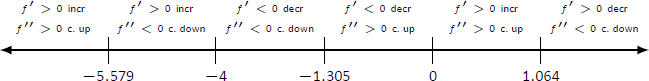
- We place the values
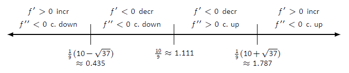
Figure
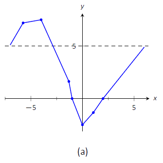
- We plot the appropriate points on axes as shown in Figure
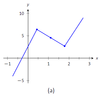
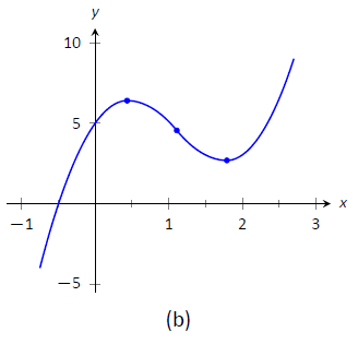
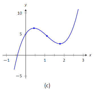
Figure
Example
Sketch
Solution
We again follow the steps outlined in Key Idea 4.
- In determining the domain, we assume it is all real numbers and looks for restrictions. We find that at
- To find the critical values of
- To find the possible points of inflection, we find
- The vertical asymptotes of
- There is a horizontal asymptote of
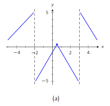
- We place the values
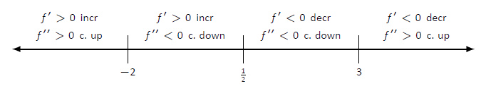
FIgure
- In Figure
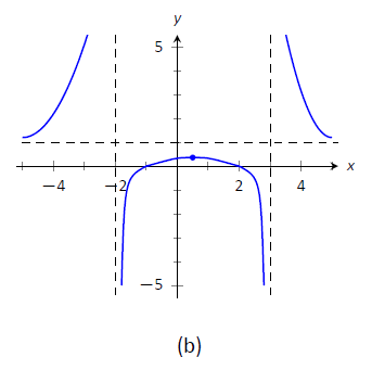
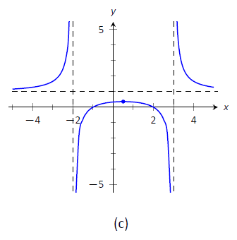
Figure
Figure
Example
Sketch
Solution
We again follow Key Idea 4
- We assume that the domain of
- We find the critical values of
- We find the possible points of inflection by solving
- There are no vertical asymptotes.
- We have a horizontal asymptote of
- We place the critical points and possible points on a number line as shown in Figure
Figure
- In Figure
Figure
In each of our examples, we found a few, significant points on the graph of
Why are computer graphics so good? It is not because computers are "smarter" than we are. Rather, it is largely because computers are much faster at computing than we are. In general, computers graph functions much like most students do when first learning to draw graphs: they plot equally spaced points, then connect the dots using lines. By using lots of points, the connecting lines are short and the graph looks smooth.
This does a fine job of graphing in most cases (in fact, this is the method used for many graphs in this text). However, in regions where the graph is very "curvy," this can generate noticeable sharp edges on the graph unless a large number of points are used. High quality computer algebra systems, such as Mathematica, use special algorithms to plot lots of points only where the graph is "curvy.''
In Figure
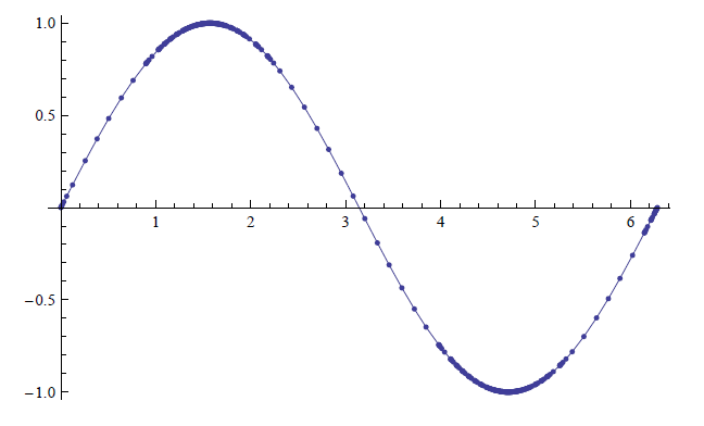
Figure
How does Mathematica know where the graph is "curvy"? Calculus. When we study curvature in a later chapter, we will see how the first and second derivatives of a function work together to provide a measurement of "curviness." Mathematica employs algorithms to determine regions of "high curvature"' and plots extra points there.
Again, the goal of this section is not "How to graph a function when there is no computer to help.'' Rather, the goal is "Understand that the shape of the graph of a function is largely determined by understanding the behavior of the function at a few key places." In Example
There are many applications of our understanding of derivatives beyond curve sketching. The next chapter explores some of these applications, demonstrating just a few kinds of problems that can be solved with a basic knowledge of differentiation.
Contributors and Attributions
Gregory Hartman (Virginia Military Institute). Contributions were made by Troy Siemers and Dimplekumar Chalishajar of VMI and Brian Heinold of Mount Saint Mary's University. This content is copyrighted by a Creative Commons Attribution - Noncommercial (BY-NC) License. http://www.apexcalculus.com/
Integrated by Justin Marshall.