5.4: The Fundamental Theorem of Calculus

The Fundamental Theorem of Calculus

Let $f(t)$ be a continuous function defined on $[a,b]$. The definite integral $\displaystyle \int_a^b f(x)\,dx$ is the "area under $f$" on $[a,b]$. We can turn this concept into a function by letting the upper (or lower) bound vary.

Let $\displaystyle F(x) = \int_a^x f(t) \,dt$. It computes the area under $f$ on $[a,x]$ as illustrated in Figure $\PageIndex{1}$. We can study this function using our knowledge of the definite integral. For instance, $F(a)=0$ since $\displaystyle \int_a^af(t) \,dt=0$.

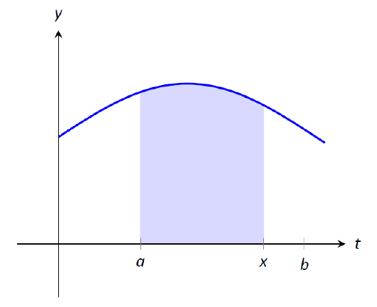
Figure $\PageIndex{1}$: The area of the shaded region is $\displaystyle F(x) = \int_a^x f(t) \,dt$.

We can also apply calculus ideas to $F(x)$; in particular, we can compute its derivative. While this may seem like an innocuous thing to do, it has far--reaching implications, as demonstrated by the fact that the result is given as an important theorem.

Theorem $\PageIndex{1}$: The Fundamental Theorem of Calculus, Part 1

Let $f$ be continuous on $[a,b]$ and let $\displaystyle F(x) = \int_a^x f(t) \,dt$. Then $F$ is a differentiable function on $(a,b)$, and

$$F'(x)=f(x).$$

Initially this seems simple, as demonstrated in the following example.

Example $\PageIndex{1}$: Using the Fundamental Theorem of Calculus, Part 1

Let $\displaystyle F(x) = \int_{-5}^x (t^2+\sin t) \,dt$. What is $F'(x)$?}

Solution

Using the Fundamental Theorem of Calculus, we have $F'(x) = x^2+\sin x$.

This simple example reveals something incredible: $F(x)$ is an antiderivative of $x^2+\sin x$! Therefore, $F(x) = \frac13x^3-\cos x+C$ for some value of $C$. (We can find $C$, but generally we do not care. We know that $F(-5)=0$, which allows us to compute $C$. In this case, $C=\cos(-5)+\frac{125}3$.)

We have done more than found a complicated way of computing an antiderivative. Consider a function $f$ defined on an open interval containing $a$, $b$ and $c$. Suppose we want to compute $\displaystyle \int_a^b f(t) \,dt$. First, let $\displaystyle F(x) = \int_c^x f(t)\,dt$. Using the properties of the definite integral found in Theorem 5.2.1, we know

$$\begin{align}\int_a^b f(t) \,dt&= \int_a^c f(t) \,dt+ \int_c^b f(t) \,dt \\ &= -\int_c^a f(t) \,dt + \int_c^b f(t) \,dt \\ &=-F(a) + F(b)\\&= F(b) - F(a). \end{align}$$

We now see how indefinite integrals and definite integrals are related: we can evaluate a definite integral using antiderivatives! This is the second part of the Fundamental Theorem of Calculus.

Theorem $\PageIndex{2}$: The Fundamental Theorem of Calculus, Part 2

Let $f$ be continuous on $[a,b]$ and let $F$ be any antiderivative of $f$. Then

$$\int_a^b f(x)\,dx = F(b) - F(a).$$

Example $\PageIndex{2}$: Using the Fundamental Theorem of Calculus, Part 2

We spent a great deal of time in the previous section studying $\int_0^4(4x-x^2)\,dx$. Using the Fundamental Theorem of Calculus, evaluate this definite integral.

Solution

We need an antiderivative of $f(x)=4x-x^2$. All antiderivatives of $f$ have the form $F(x) = 2x^2-\frac13x^3+C$; for simplicity, choose $C=0$.

The Fundamental Theorem of Calculus states

$$\int_0^4(4x-x^2)\,dx = F(4)-F(0) = \big(2(4)^2-\frac134^3\big)-\big(0-0\big) = 32-\frac{64}3 = 32/3.$$

This is the same answer we obtained using limits in the previous section, just with much less work.

Notation: A special notation is often used in the process of evaluating definite integrals using the Fundamental Theorem of Calculus. Instead of explicitly writing $F(b)-F(a)$, the notation $F(x)\Big|_a^b$ is used. Thus the solution to Example $\PageIndex{2}$ would be written as:

$$\int_0^4(4x-x^2)\,dx = \left.\left(2x^2-\frac13x^3\right)\right|_0^4 = \big(2(4)^2-\frac134^3\big)-\big(0-0\big) = 32/3.$$

The Constant $C$: Any antiderivative $F(x)$ can be chosen when using the Fundamental Theorem of Calculus to evaluate a definite integral, meaning any value of $C$ can be picked. The constant always cancels out of the expression when evaluating $F(b)-F(a)$, so it does not matter what value is picked. This being the case, we might as well let $C=0$.

Example $\PageIndex{3}$: Using the Fundamental Theorem of Calculus, Part 2

Evaluate the following definite integrals.

$$1.\ \int_{-2}^2 x^3\,dx \quad 2.\ \int_0^\pi \sin x\,dx \qquad 3.\ \int_0^5 e^t \,dt \qquad 4.\ \int_4^9 \sqrt{u}\ du\qquad 5.\ \int_1^5 2\,dx$$

Solution

1. $\displaystyle \int_{-2}^2 x^3\,dx = \left.\frac14x^4\right|_{-2}^2 = \left(\frac142^4\right) - \left(\frac14(-2)^4\right) = 0.$
2. $\displaystyle \int_0^\pi \sin x\,dx = -\cos x\Big|_0^\pi = -\cos \pi- \big(-\cos 0\big) = 1+1=2.$
   (This is interesting; it says that the area under one "hump" of a sine curve is 2.)
3. $\displaystyle \int_0^5e^t \,dt = e^t\Big|_0^5 = e^5 - e^0 = e^5-1 \approx 147.41.$
4. $\displaystyle \int_4^9 \sqrt{u}\ du = \int_4^9 u^\frac12\ du = \left.\frac23u^\frac32\right|_4^9 = \frac23\left(9^\frac32-4^\frac32\right) = \frac23\big(27-8\big) =\frac{38}3.$
5. $\displaystyle \int_1^5 2\,dx = 2x\Big|_1^5 = 2(5)-2=2(5-1)=8.$

This integral is interesting; the integrand is a constant function, hence we are finding the area of a rectangle with width $(5-1)=4$ and height 2. Notice how the evaluation of the definite integral led to $2(4)=8$.

In general, if $c$ is a constant, then $\displaystyle \int_a^b c\,dx = c(b-a)$.

Understanding Motion with the Fundamental Theorem of Calculus

We established, starting with Key Idea 1, that the derivative of a position function is a velocity function, and the derivative of a velocity function is an acceleration function. Now consider definite integrals of velocity and acceleration functions. Specifically, if $v(t)$ is a velocity function, what does $\displaystyle \int_a^b v(t) \,dt$ mean?

The Fundamental Theorem of Calculus states that

$$\int_a^b v(t) \,dt = V(b) - V(a),$$

where $V(t)$ is any antiderivative of $v(t)$. Since $v(t)$ is a velocity function, $V(t)$ must be a position function, and $V(b) - V(a)$ measures a change in position, or displacement.

Example $\PageIndex{4}$: Finding displacement

A ball is thrown straight up with velocity given by $v(t) = -32t+20$ft/s, where $t$ is measured in seconds. Find, and interpret, $\displaystyle \int_0^1 v(t) \,dt.$}

Solution

Using the Fundamental Theorem of Calculus, we have

$$\begin{align} \int_0^1 v(t) \,dt &= \int_0^1 (-32t+20) \,dt \\ &= -16t^2 + 20t\Big|_0^1 \\ &= 4. \end{align}$$

Thus if a ball is thrown straight up into the air with velocity $v(t) = -32t+20$, the height of the ball, 1 second later, will be 4 feet above the initial height. (Note that the ball has traveled much farther. It has gone up to its peak and is falling down, but the difference between its height at $t=0$ and $t=1$ is 4 ft.

Integrating a rate of change function gives total change. Velocity is the rate of position change; integrating velocity gives the total change of position, i.e., displacement.

Integrating a speed function gives a similar, though different, result. Speed is also the rate of position change, but does not account for direction. So integrating a speed function gives total change of position, without the possibility of "negative position change." Hence the integral of a speed function gives distance traveled.

As acceleration is the rate of velocity change, integrating an acceleration function gives total change in velocity. We do not have a simple term for this analogous to displacement. If $a(t) = 5 \text{ miles}/\text{h}^2$ and $t$ is measured in hours, then

$$\int_0^3 a(t) \,dt = 15$$

means the velocity has increased by 15 m/h from $t=0$ to $t=3$.

The Fundamental Theorem of Calculus and the Chain Rule

Part 1 of the Fundamental Theorem of Calculus (FTC) states that given $\displaystyle F(x) = \int_a^x f(t) \,dt$, $F'(x) = f(x)$. Using other notation, $\frac{d}{\,dx}\big(F(x)\big) = f(x)$. While we have just practiced evaluating definite integrals, sometimes finding antiderivatives is impossible and we need to rely on other techniques to approximate the value of a definite integral. Functions written as $\displaystyle F(x) = \int_a^x f(t) \,dt$ are useful in such situations.

It may be of further use to compose such a function with another. As an example, we may compose $F(x)$ with $g(x)$ to get

$$F\big(g(x)\big) = \int_a^{g(x)} f(t) \,dt.$$

What is the derivative of such a function? The Chain Rule can be employed to state

$$\frac{d}{\,dx}\Big(F\big(g(x)\big)\Big) = F'\big(g(x)\big)g'(x) = f\big(g(x)\big)g'(x).$$

An example will help us understand this.

Example $\PageIndex{4}$: The FTC, Part 1, and the Chain Rule

Find the derivative of $\displaystyle F(x) = \int_2^{x^2} \ln t \,dt$.

Solution

We can view $F(x)$ as being the function $\displaystyle G(x) = \int_2^x \ln t \,dt$ composed with $g(x) = x^2$; that is, $F(x) = G\big(g(x)\big)$. The Fundamental Theorem of Calculus states that $G'(x) = \ln x$. The Chain Rule gives us

$$\begin{align} F'(x) &= G'\big(g(x)\big) g'(x) \\ &= \ln (g(x)) g'(x) \\ &= \ln (x^2) 2x \\ &=2x\ln x^2 \end{align}$$

Normally, the steps defining $G(x)$ and $g(x)$ are skipped.

Practice this once more.

Example $\PageIndex{5}$: The FTC, Part 1, and the Chain Rule

Find the derivative of $\displaystyle F(x) = \int_{\cos x}^5 t^3 \,dt.$

Solution

Note that $\displaystyle F(x) = -\int_5^{\cos x} t^3 \,dt$. Viewed this way, the derivative of $F$ is straightforward:

$$F'(x) = \sin x \cos^3 x.$$

Area Between Curves

Consider continuous functions $f(x)$ and $g(x)$ defined on $[a,b]$, where $f(x) \geq g(x)$ for all $x$ in $[a,b]$, as demonstrated in Figure $\PageIndex{2}$. What is the area of the shaded region bounded by the two curves over $[a,b]$?

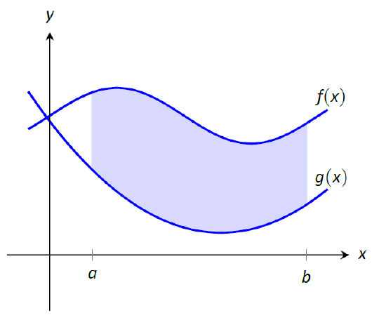
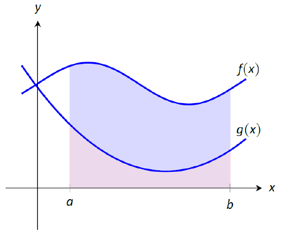
Figure $\PageIndex{2}$: Finding the area bounded by two functions on an interval; it is found by subtracting the area under $g$ from the area under $f$.

The area can be found by recognizing that this area is "the area under $f$ $-$ the area under $g$." Using mathematical notation, the area is

$$\int_a^b f(x)\,dx - \int_a^b g(x)\,dx.$$

Properties of the definite integral allow us to simplify this expression to

$$\int_a^b\big(f(x) - g(x)\big)\,dx.$$

Theorem $\PageIndex{3}$: Area Between Curves

Let $f(x)$ and $g(x)$ be continuous functions defined on $[a,b]$ where $f(x)\geq g(x)$ for all $x$ in $[a,b]$. The area of the region bounded by the curves $y=f(x)$, $y=g(x)$ and the lines $x=a$ and $x=b$ is

$$\int_a^b \big(f(x)-g(x)\big)\,dx.$$

Example $\PageIndex{6}$: Finding area between curves

Find the area of the region enclosed by $y=x^2+x-5$ and $y=3x-2$.

Solution

It will help to sketch these two functions, as done in Figure $\PageIndex{3}$.

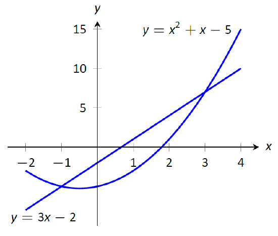
Figure $\PageIndex{3}$: Sketching the region enclosed by $y=x^2+x-5$ and $y=3x-2$ in Example $\PageIndex{6}$

The region whose area we seek is completely bounded by these two functions; they seem to intersect at $x=-1$ and $x=3$. To check, set $x^2+x-5=3x-2$ and solve for $x$:

$$\begin{align} x^2+x-5 &= 3x-2 \\ (x^2+x-5) - (3x-2) &= 0\\ x^2-2x-3 &= 0\\ (x-3)(x+1) &= 0\\ x&=-1,\ 3. \end{align}$$

Following Theorem $\PageIndex{3}$, the area is

$$\begin{align}\int_{-1}^3\big(3x-2 -(x^2+x-5)\big)\,dx &= \int_{-1}^3 (-x^2+2x+3)\,dx \\ &=\left.\left(-\frac13x^3+x^2+3x\right)\right|_{-1}^3 \\ &=-\frac13(27)+9+9-\left(\frac13+1-3\right)\\ &= 10\frac23 = 10.\overline{6} \end{align}$$

The Mean Value Theorem and Average Value

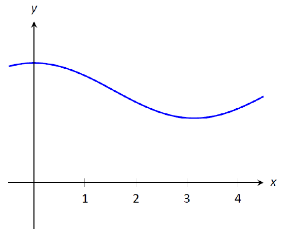
Figure $\PageIndex{4}$: A graph of a function $f$ to introduce the Mean Value Theorem.

Consider the graph of a function $f$ in Figure $\PageIndex{4}$ and the area defined by $\displaystyle \int_1^4 f(x)\,dx$. Three rectangles are drawn in Figure $\PageIndex{5}$; in (a), the height of the rectangle is greater than $f$ on $[1,4]$, hence the area of this rectangle is is greater than $\displaystyle \int_0^4 f(x)\,dx$.

In (b), the height of the rectangle is smaller than $f$ on $[1,4]$, hence the area of this rectangle is less than $\displaystyle \int_1^4 f(x)\,dx$.

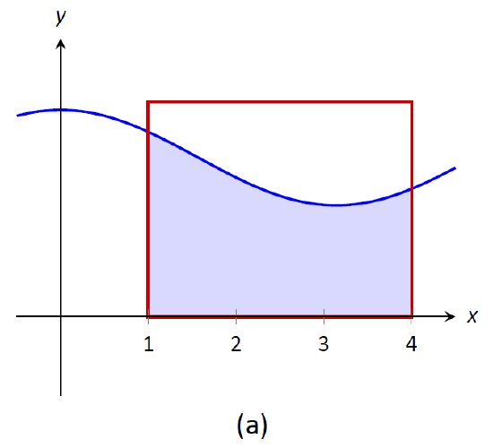
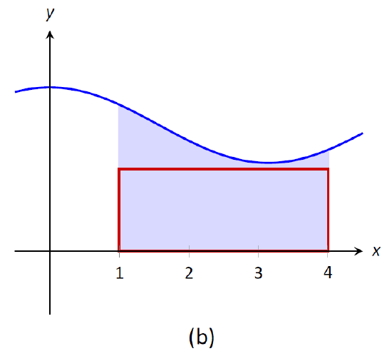
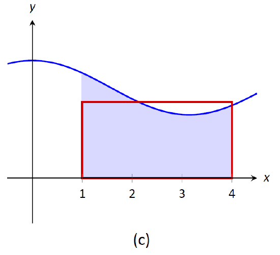
Figure $\PageIndex{5}$: Differently sized rectangles give upper and lower bounds on $\displaystyle \int_1^4 f(x)\,dx$; the last rectangle matches the area exactly.

Finally, in (c) the height of the rectangle is such that the area of the rectangle is exactly that of $\displaystyle \int_0^4 f(x)\,dx$. Since rectangles that are "too big", as in (a), and rectangles that are "too little," as in (b), give areas greater/lesser than $\displaystyle \int_1^4 f(x)\,dx$, it makes sense that there is a rectangle, whose top intersects $f(x)$ somewhere on $[1,4]$, whose area is exactly that of the definite integral.

We state this idea formally in a theorem.

Theorem $\PageIndex{4}$: The Mean Value Theorem of Integration

Let $f$ be continuous on $[a,b]$. There exists a value $c$ in $[a,b]$ such that

$$\int_a^bf(x)\,dx = f(c)(b-a).$$

This is an existential statement; $c$ exists, but we do not provide a method of finding it. Theorem $\PageIndex{4}$ is directly connected to the Mean Value Theorem of Differentiation, given as Theorem 3.2.1; we leave it to the reader to see how.

We demonstrate the principles involved in this version of the Mean Value Theorem in the following example.

Example $\PageIndex{7}$: Using the Mean Value Theorem

Consider $\displaystyle \int_0^\pi \sin x\,dx$. Find a value $c$ guaranteed by the Mean Value Theorem.

Solution

We first need to evaluate $\displaystyle \int_0^\pi \sin x\,dx$. (This was previously done in Example $\PageIndex{3}$)

$$\int_0^\pi\sin x\,dx = -\cos x \Big|_0^\pi = 2.$$

Thus we seek a value $c$ in $[0,\pi]$ such that $\pi\sin c =2$.

$$\pi\sin c = 2\ \ \Rightarrow\ \ \sin c = 2/\pi\ \ \Rightarrow\ \ c = \arcsin(2/\pi) \approx 0.69.$$

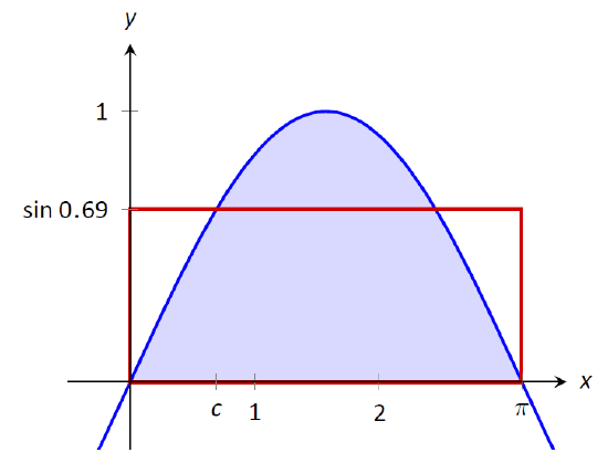
Figure $\PageIndex{6}$: A graph of $y=\sin x$ on $[0,\pi]$ and the rectangle guaranteed by the Mean Value Theorem.

In Figure $\PageIndex{6}$ $\sin x$ is sketched along with a rectangle with height $\sin (0.69)$. The area of the rectangle is the same as the area under $\sin x$ on $[0,\pi]$.

Let $f$ be a function on $[a,b]$ with $c$ such that $\displaystyle f(c)(b-a) = \int_a^bf(x)\,dx$. Consider $\displaystyle \int_a^b\big(f(x)-f(c)\big)\,dx$:

$$\begin{align} \int_a^b\big(f(x)-f(c)\big)\,dx &= \int_a^b f(x) - \int_a^b f(c)\,dx\\ &= f(c)(b-a) - f(c)(b-a) \\ &= 0. \end{align}$$

When $f(x)$ is shifted by $-f(c)$, the amount of area under $f$ above the $x$-axis on $[a,b]$ is the same as the amount of area below the $x$-axis above $f$; see Figure $\PageIndex{7}$ for an illustration of this. In this sense, we can say that $f(c)$ is the average value of $f$ on $[a,b]$.

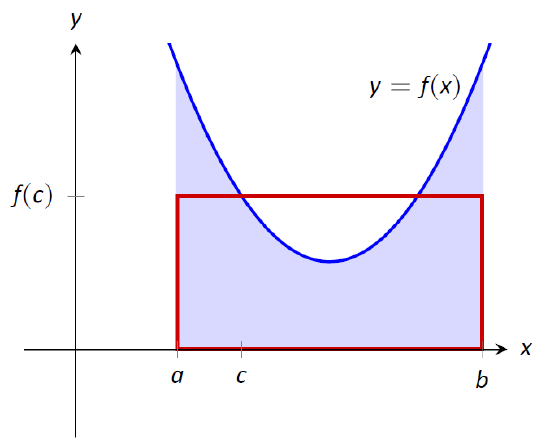
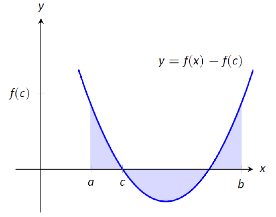
Figure $\PageIndex{7}$: On the left, a graph of $y=f(x)$ and the rectangle guaranteed by the Mean Value Theorem. On the right, $y=f(x)$ is shifted down by $f(c)$; the resulting "area under the curve" is 0.

The value $f(c)$ is the average value in another sense. First, recognize that the Mean Value Theorem can be rewritten as

$$f(c) = \frac{1}{b-a}\int_a^b f(x)\,dx,$$

for some value of $c$ in $[a,b]$. Next, partition the interval $[a,b]$ into $n$ equally spaced subintervals, $a=x_1 < x_2 < \ldots < x_{n+1}=b$ and choose any $c_i$ in $[x_i,x_{i+1}]$. The average of the numbers $f(c_1)$, $f(c_2)$, $\ldots$, $f(c_n)$ is:

$$\frac1n\Big(f(c_1) + f(c_2) + \ldots + f(c_n)\Big) = \frac1n\sum_{i=1}^n f(c_i).$$

Multiply this last expression by 1 in the form of $\frac{(b-a)}{(b-a)}$:

$$\begin{align} \frac1n\sum_{i=1}^n f(c_i) &= \sum_{i=1}^n f(c_i)\frac1n \\ &= \sum_{i=1}^n f(c_i)\frac1n \frac{(b-a)}{(b-a)} \\ &=\frac{1}{b-a} \sum_{i=1}^n f(c_i)\,\Delta x\quad \text{(where $\Delta x = (b-a)/n$)} \end{align}$$

Now take the limit as $n\to\infty$:

$$\lim_{n\to\infty} \frac{1}{b-a} \sum_{i=1}^n f(c_i)\,\Delta x\quad = \quad \frac{1}{b-a} \int_a^b f(x)\,dx\quad = \quad f(c).$$

This tells us this: when we evaluate $f$ at $n$ (somewhat) equally spaced points in $[a,b]$, the average value of these samples is $f(c)$ as $n\to\infty$.

This leads us to a definition.

Definition $\PageIndex{1}$: The Average Value of $f$ on $[a,b]$

Let $f$ be continuous on $[a,b]$. The average value of $f$ on $[a,b]$ is $f(c)$, where $c$ is a value in $[a,b]$ guaranteed by the Mean Value Theorem. I.e.,

$$\text{Average Value of \(f\) on \([a,b]\)} = \frac{1}{b-a}\int_a^b f(x)\,dx.$$

An application of this definition is given in the following example.

Example $\PageIndex{8}$: Finding the average value of a function

An object moves back and forth along a straight line with a velocity given by $v(t) = (t-1)^2$ on $[0,3]$, where $t$ is measured in seconds and $v(t)$ is measured in ft/s.

What is the average velocity of the object?

Solution

By our definition, the average velocity is:

$$\frac{1}{3-0}\int_0^3 (t-1)^2 \,dt =\frac13 \int_0^3 \big(t^2-2t+1\big) \,dt = \left.\frac13\left(\frac13t^3-t^2+t\right)\right|_0^3 = 1\text{ ft/s}.$$

We can understand the above example through a simpler situation. Suppose you drove 100 miles in 2 hours. What was your average speed? The answer is simple: $\text{displacement}/\text{time} = 100 \;\text{miles}/2\;\text{hours} = 50 mph$.

What was the displacement of the object in Example $\PageIndex{8}$? We calculate this by integrating its velocity function: $\displaystyle \int_0^3 (t-1)^2 \,dt = 3$ ft. Its final position was 3 feet from its initial position after 3 seconds: its average velocity was 1 ft/s.

This section has laid the groundwork for a lot of great mathematics to follow. The most important lesson is this: definite integrals can be evaluated using antiderivatives. Since the previous section established that definite integrals are the limit of Riemann sums, we can later create Riemann sums to approximate values other than "area under the curve," convert the sums to definite integrals, then evaluate these using the Fundamental Theorem of Calculus. This will allow us to compute the work done by a variable force, the volume of certain solids, the arc length of curves, and more.

The downside is this: generally speaking, computing antiderivatives is much more difficult than computing derivatives. The next chapter is devoted to techniques of finding antiderivatives so that a wide variety of definite integrals can be evaluated. Before that, the next section explores techniques of approximating the value of definite integrals beyond using the Left Hand, Right Hand and Midpoint Rules.

Contributors and Attributions

• Gregory Hartman (Virginia Military Institute). Contributions were made by Troy Siemers and Dimplekumar Chalishajar of VMI and Brian Heinold of Mount Saint Mary's University. This content is copyrighted by a Creative Commons Attribution - Noncommercial (BY-NC) License. http://www.apexcalculus.com/

• Integrated by Justin Marshall.