5.5: Numerical Integration

The Fundamental Theorem of Calculus gives a concrete technique for finding the exact value of a definite integral. That technique is based on computing antiderivatives. Despite the power of this theorem, there are still situations where we must approximate the value of the definite integral instead of finding its exact value. The first situation we explore is where we cannot compute the antiderivative of the integrand. The second case is when we actually do not know the integrand, but only its value when evaluated at certain points.

An elementary function is any function that is a combination of polynomials, \(n^{\text{th}}\) roots, rational, exponential, logarithmic and trigonometric functions. We can compute the derivative of any elementary function, but there are many elementary functions of which we cannot compute an antiderivative. For example, the following functions do not have antiderivatives that we can express with elementary functions:

$$e^{-x^2}, \quad \sin(x^3)\quad \text{and} \quad \frac{\sin x}{x}.\]

The simplest way to refer to the antiderivatives of \(e^{-x^2}\) is to simply write \(\int e^{-x^2}\ dx\).

This section outlines three common methods of approximating the value of definite integrals. We describe each as a systematic method of approximating area under a curve. By approximating this area accurately, we find an accurate approximation of the corresponding definite integral.

We will apply the methods we learn in this section to the following definite integrals:

$$ \int_0^1 e^{-x^2} \ dx, \quad \int_{-\frac{\pi}{4}}^{\frac{\pi}{2}} \sin(x^3) \ dx, \quad \text{and} \quad \int_{0.5}^{4\pi} \frac{\sin(x)}{x} \ dx,\]

as pictured in Figure \(\PageIndex{1}\).

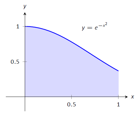
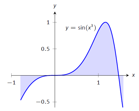
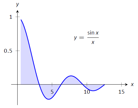
Figure \(\PageIndex{1}\): Graphically representing three definite integrals that cannot be evaluated using antiderivatives.

The Left and Right Hand Rule Methods

In Section 5.3 we addressed the problem of evaluating definite integrals by approximating the area under the curve using rectangles. We revisit those ideas here before introducing other methods of approximating definite integrals.

We start with a review of notation. Let \(f\) be a continuous function on the interval \([a,b]\). We wish to approximate \(\int_a^b f(x)\ dx\). We partition \([a,b]\) into \(n\) equally spaced subintervals, each of length \(dx = \frac{b-a}{n}\). The endpoints of these subintervals are labeled as

$$x_1=a,\ x_2 = a+dx,\ x_3 = a+ 2dx,\ \ldots,\ x_i = a+(i-1)\ dx,\ \ldots,\ x_{n+1} = b.\]

Key Idea 8 states that to use the Left Hand Rule we use the summation \( \sum_{i=1}^n f(x_i)\ dx\) and to use the Right Hand Rule we use \( \sum_{i=1}^n f(x_{i+1})\ dx\). We review the use of these rules in the context of examples.

Example \(\PageIndex{1}\): Approximating definite integrals with rectangles

Approximate \( \int_0^1e^{-x^2}\ dx\) using the Left and Right Hand Rules with 5 equally spaced subintervals.

Solution

We begin by partitioning the interval \([0,1]\) into 5 equally spaced intervals. We have \(dx = \frac{1-0}5 = 1/5=0.2\), so $$x_1 = 0,\ x_2 = 0.2,\ x_3 = 0.4,\ x_4 = 0.6,\ x_5 = 0.8,\ \text{and}\ x_6 = 1.\]

Using the Left Hand Rule, we have:

\[\begin{align} \sum_{i=1}^n f(x_i)\ dx &= \big(f(x_1)+f(x_2) + f(x_3) + f(x_4) + f(x_5)\big)\ dx \\ &= \big(f(0) + f(0.2) + f(0.4) + f(0.6) + f(0.8)\big)\ dx \\ &\approx \big(1+0.961 + 0.852 + 0.698 + 0.527)(0.2)\\ &\approx 0.808.\end{align}\]

Using the Right Hand Rule, we have:

\[\begin{align} \sum_{i=1}^n f(x_{i+1})\ dx &= \big(f(x_2) + f(x_3) + f(x_4) + f(x_5)+f(x_6)\big)\ dx \\ &= \big(f(0.2) + f(0.4)+ f(0.6) + f(0.8)+f(1)\big)\ dx \\ &\approx \big(0.961 +0.852 + 0.698 + 0.527 + 0.368)(0.2)\\ &\approx 0.681.
\end{align}\]

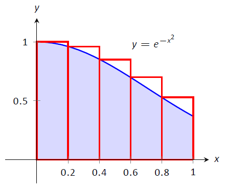
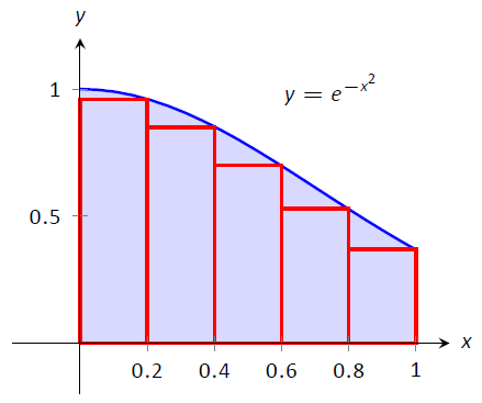
Figure \(\PageIndex{2}\): Approximating \(\int_0^1e^{-x^2}\ dx\) in Example \(\PageIndex{1}\)

Figure \(\PageIndex{2}\) shows the rectangles used in each method to approximate the definite integral. These graphs show that in this particular case, the Left Hand Rule is an over approximation and the Right Hand Rule is an under approximation. To get a better approximation, we could use more rectangles, as we did in Section 3.1. We could also average the Left and Right Hand Rule results together, giving

$$ \frac{0.808 + 0.681}{2} = 0.7445.\]

The actual answer, accurate to 4 places after the decimal, is 0.7468, showing our average is a good approximation.

Example \(\PageIndex{2}\): Approximating definite integrals with rectangles

Approximate \(\int_{-\frac{\pi}4}^{\frac{\pi}2} \sin (x^3)\ dx\) using the Left and Right Hand Rules with 10 equally spaced subintervals.

Solution

We begin by finding \Delta x:

$$\frac{b-a}{n} = \frac{\pi/2 - (-\pi/4)}{10} = \frac{3\pi}{40}\approx 0.236.\]

It is useful to write out the endpoints of the subintervals in a table; in Table \(\PageIndex{1}\), we give the exact values of the endpoints, their decimal approximations, and decimal approximations of \(\sin(x^3)\) evaluated at these points.

Table \(\PageIndex{1}\): Table of values used to approximate \(\int_{-\frac{\pi}4}^{\frac{\pi}2}\sin(x^3)\ dx\) in Example \(\PageIndex{1}\).

\(x_i\)	Exact	Approx.	\(\sin(x_i^3)\)
\(x_1\)	\(-\pi/4\)	\(-0.785\)	\(-0.466\)
\(x_2\)	\(-7 \pi/40\)	\(-0.550\)	\(-0.165\)
\(x_3\)	\(-{\pi }/{10}\)	\(-0.314\)	\(-0.031\)
\(x_4\)	\(-{\pi }/{40}\)	\(-0.0785\)	\(0\)
\(x_5\)	\({\pi }/{20}\)	0.157	0.004
\(x_6\)	\({\pi }/{8}\)	0.393	0.061
\(x_7\)	\({\pi }/{5}\)	0.628	0.246
\(x_8\)	\({11 \pi }/{40}\)	0.864	0.601
\(x_9\)	\({7 \pi }/{20}\)	1.10	0.971
\(x_{10}\)	\({17 \pi }/{40}\)	1.34	0.690
\(x_{11}\)	\({\pi}/{2}\)	1.57	\(-0.670\)

Once this table is created, it is straightforward to approximate the definite integral using the Left and Right Hand Rules. (Note: the table itself is easy to create, especially with a standard spreadsheet program on a computer. The last two columns are all that are needed.) The Left Hand Rule sums the first 10 values of \(\sin(x_i^3)\) and multiplies the sum by \(dx\); the Right Hand Rule sums the last 10 values of \(\sin(x_i^3)\) and multiplies by \(dx\). Therefore we have:

Left Hand Rule: \(\int_{-\frac{\pi}4}^{\frac{\pi}2}\sin(x^3)\ dx \approx (1.91)(0.236) = 0.451.\)

Right Hand Rule: \(\int_{-\frac{\pi}4}^{\frac{\pi}2}\sin(x^3)\ dx \approx (1.71)(0.236) = 0.404.\)

Average of the Left and Right Hand Rules: 0.4275.

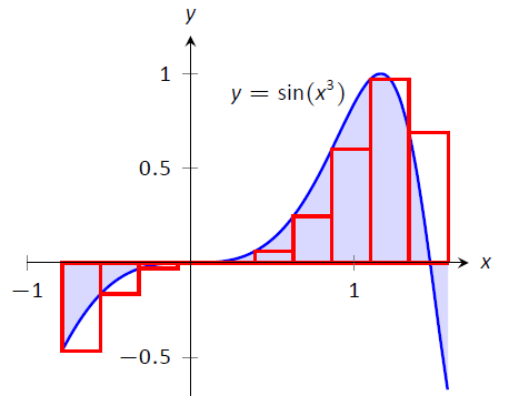
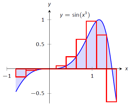
Figure \(\PageIndex{3}\): \(\int_{-\frac{\pi}4}^{\frac{\pi}2}\sin(x^3)\ dx\) in Example \(\PageIndex{2}\)

The actual answer, accurate to 3 places after the decimal, is 0.460. Our approximations were once again fairly good. The rectangles used in each approximation are shown in Figure \(\PageIndex{3}\). It is clear from the graphs that using more rectangles (and hence, narrower rectangles) should result in a more accurate approximation.

The Trapezoidal Rule

In Example \(\PageIndex{1}\) we approximated the value of \(\int_0^1 e^{-x^2}\ dx\) with 5 rectangles of equal width. Figure \(\PageIndex{2}\) shows the rectangles used in the Left and Right Hand Rules. These graphs clearly show that rectangles do not match the shape of the graph all that well, and that accurate approximations will only come by using lots of rectangles.

Instead of using rectangles to approximate the area, we can instead use trapezoids. In Figure \(\PageIndex{4}\), we show the region under \(f(x) = e^{-x^2}\) on \([0,1]\) approximated with 5 trapezoids of equal width; the top "corners" of each trapezoid lies on the graph of \(f(x)\). It is clear from this figure that these trapezoids more accurately approximate the area under \(f\) and hence should give a better approximation of \(\int_0^1 e^{-x^2}\ dx\). (In fact, these trapezoids seem to give a great approximation of the area!)

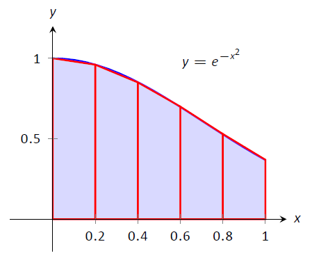
Figure \(\PageIndex{4}\): Approximating \(\int_0^1 e^{-x^2}\ dx\) using 5 trapezoids of equal widths.

The formula for the area of a trapezoid is given in Figure \(\PageIndex{5}\). We approximate \(\int_0^1 e^{-x^2}\ dx\) with these trapezoids in the following example.

Example \(\PageIndex{3}\): Approximating definite integrals using trapezoids

Use 5 trapezoids of equal width to approximate \(\int_0^1e^{-x^2}\ dx\).

Solution

To compute the areas of the 5 trapezoids in Figure \(\PageIndex{6}\), it will again be useful to create a table of values as shown in Table \(\PageIndex{2}\).

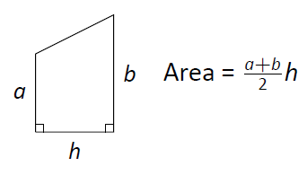
Figure \(\PageIndex{5}\): The area of a trapezoid

Table \(\PageIndex{2}\): A table of values of \(e^{-x^2}\).

\(x_i\)	\(e^{-x_i^2}\)
0	1
0.2	0.961
0.4	0.852
0.6	0.698
0.8	0.527
1	0.368

The leftmost trapezoid has legs of length 1 and 0.961 and a height of 0.2. Thus, by our formula, the area of the leftmost trapezoid is:

$$ \frac{1+0.961}{2}(0.2) = 0.1961.\]

Moving right, the next trapezoid has legs of length 0.961 and 0.852 and a height of 0.2. Thus its area is:

$\frac{0.961+0.852}2(0.2) = 0.1813.\]

The sum of the areas of all 5 trapezoids is:

\[\begin{align} \frac{1+0.961}{2}(0.2) + \frac{0.961+0.852}2(0.2)+\frac{0.852+0.698}2(0.2)&+ \\ \frac{0.698+0.527}2(0.2)+\frac{0.527+0.368}2(0.2)&= 0.7445. \end{align}\]

We approximate \(\int_0^1 e^{-x^2}\ dx \approx 0.7445.\)

There are many things to observe in this example. Note how each term in the final summation was multiplied by both 1/2 and by \(dx = 0.2\). We can factor these coefficients out, leaving a more concise summation as:

$$\frac12(0.2)\Big[(1+0.961) + (0.961+0.852) + (0.852+0.698) + ( 0.698+ 0.527) +(0.527 + 0.368)\Big].\]

Now notice that all numbers except for the first and the last are added twice. Therefore we can write the summation even more concisely as

$$\frac{0.2}{2}\Big[1 + 2(0.961+0.852+0.698+0.527) + 0.368\Big].\]

This is the heart of the Trapezoidal Rule, wherein a definite integral \(\int_a^b f(x) \ dx\) is approximated by using trapezoids of equal widths to approximate the corresponding area under \(f\). Using \(n\) equally spaced subintervals with endpoints \(x_1\), \(x_2\), \(\ldots\), \(x_{n+1}\), we again have \( \Delta x = \frac{b-a}n\). Thus:

\[\begin{align} \int_a^b f(x)\ dx & \approx \sum_{i=1}^n \frac{f(x_i)+f(x_{i+1})}2\ dx \\ & = \frac{\ dx}2 \sum_{i=1}^n \big(f(x_i)+f(x_{i+1})\big)\\ & = \frac{\ dx}2\Big[f(x_1)+ 2\sum_{i=2}^n f(x_i) + f(x_{n+1})\Big].\end{align}\]

Example \(\PageIndex{4}\): Using the Trapezoidal Rule

Revisit Example \(\PageIndex{4}\) and approximate \(\int_{-\frac{\pi}{4}}^{\frac{\pi}{2}} \sin (x^3)\ dx\) using the Trapezoidal Rule and 10 equally spaced subintervals.

Solution

We refer back to Table \(\PageIndex{1}\) for the table of values of \(\sin(x^3)\). Recall that \(dx = 3\pi/40 \approx 0.236\). Thus we have:

\[\begin{align*}\int_{-\frac {\pi}4}^{\frac{\pi}2} \sin (x^3)\ dx &\approx \frac{0.236}{2}\Big[-0.466 + 2\Big(-0.165+(-0.031)+\ldots+0.69\Big)+(-0.67)\Big]\\ &= 0.4275. \end{align*}\]

Notice how "quickly" the Trapezoidal Rule can be implemented once the table of values is created. This is true for all the methods explored in this section; the real work is creating a table of \(x_i\) and \(f(x_i)\) values. Once this is completed, approximating the definite integral is not difficult. Again, using technology is wise. Spreadsheets can make quick work of these computations and make using lots of subintervals easy.

Also notice the approximations the Trapezoidal Rule gives. It is the average of the approximations given by the Left and Right Hand Rules! This effectively renders the Left and Right Hand Rules obsolete. They are useful when first learning about definite integrals, but if a real approximation is needed, one is generally better off using the Trapezoidal Rule instead of either the Left or Right Hand Rule.

How can we improve on the Trapezoidal Rule, apart from using more and more trapezoids? The answer is clear once we look back and consider what we have really done so far. The Left Hand Rule is not really about using rectangles to approximate area. Instead, it approximates a function \(f\) with constant functions on small subintervals and then computes the definite integral of these constant functions. The Trapezoidal Rule is really approximating a function \(f\) with a linear function on a small subinterval, then computes the definite integral of this linear function. In both of these cases the definite integrals are easy to compute in geometric terms.

So we have a progression: we start by approximating \(f\) with a constant function and then with a linear function. What is next? A quadratic function. By approximating the curve of a function with lots of parabolas, we generally get an even better approximation of the definite integral. We call this process Simpson's Rule, named after Thomas Simpson (1710-1761), even though others had used this rule as much as 100 years prior.

Simpson's Rule

Given one point, we can create a constant function that goes through that point. Given two points, we can create a linear function that goes through those points. Given three points, we can create a quadratic function that goes through those three points (given that no two have the same \(x\)--value).

Consider three points \((x_1,y_1)\), \((x_2,y_2)\) and \((x_3,y_3)\) whose \(x\)--values are equally spaced and \(x_1<x_2<x_3\). Let \(f\) be the quadratic function that goes through these three points. It is not hard to show that

\[\int_{x_1}^{x_3} f(x)\ dx = \frac{x_3-x_1}{6}\big(y_1+4y_2+y_3\big).\]

Consider Figure \(\PageIndex{6}\). A function \(f\) goes through the 3 points shown and the parabola \(g\) that also goes through those points is graphed with a dashed line. Using our equation from above, we know exactly that $$\int_1^3 g(x) \ dx = \frac{3-1}{6}\big(3+4(1)+2\big)= 3.$$ Since \(g\) is a good approximation for \(f\) on \([1,3]\), we can state that $$\int_1^3 f(x)\ dx \approx 3.\]

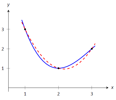
Figure \(\PageIndex{6}\): A graph of a function \(f\) and a parabola that approximates it well on \([1,3]\).

Notice how the interval \([1,3]\) was split into two subintervals as we needed 3 points. Because of this, whenever we use Simpson's Rule, we need to break the interval into an even number of subintervals.

In general, to approximate \(\int_a^b f(x)\ dx\) using Simpson's Rule, subdivide \([a,b]\) into \(n\) subintervals, where \(n\) is even and each subinterval has width \(\ dx = (b-a)/n\). We approximate \(f\) with \(n/2\) parabolic curves, using Equation \(\PageIndex{22}\) to compute the area under these parabolas. Adding up these areas gives the formula:

$$\int_a^b f(x) \ dx \approx \frac{\ dx}3\Big[f(x_1)+4f(x_2)+2f(x_3)+4f(x_4)+\ldots+2f(x_{n-1})+4f(x_n)+f(x_{n+1})\Big].\]

Note how the coefficients of the terms in the summation have the pattern 1, 4, 2, 4, 2, 4, \(\ldots\), 2, 4, 1.

Let's demonstrate Simpson's Rule with a concrete example.

Example \(\PageIndex{5}\): Using Simpson's Rule

Approximate \(\int_0^1 e^{-x^2}\ dx\) using Simpson's Rule and 4 equally spaced subintervals.

Solution

We begin by making a table of values as we have in the past, as shown in Table \(\PageIndex{3}\).

Table \(\PageIndex{3}\): A table of values to approximate \(\int_0^1e^{-x^2}\ dx\), along with a graph of the function.

\(x_i\)	\(e^{-x_i^2}\)
0	1
0.25	0.939
0.5	0.779
0.75	0.570
1	0.368

Simpson's Rule states that

$$\int_0^1e^{-x^2}\ dx \approx \frac{0.25}{3}\Big[1+4(0.939)+2(0.779)+4(0.570) + 0.368\Big] = 0.7468\overline{3}.\]

Recall in Example \(\PageIndex{1}\) we stated that the correct answer, accurate to 4 places after the decimal, was 0.7468. Our approximation with Simpson's Rule, with 4 subintervals, is better than our approximation with the Trapezoidal Rule using 5!

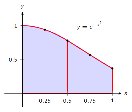
Figure \(\PageIndex{7}\): Using Simpson's Rule with \(n=4\) to approximate \(\int_0^1 e^{-x^2}\ dx\).

Figure \(\PageIndex{7}\) shows \(f(x) = e^{-x^2}\) along with its approximating parabolas, demonstrating how good our approximation is. The approximating curves are nearly indistinguishable from the actual function.

Example \(\PageIndex{6}\): Using Simpson's Rule

Approximate \(\int_{-\frac{\pi}4}^{\frac{\pi}2} \sin (x^3)\ dx\) using Simpson's Rule and 10 equally spaced intervals.

Solution

Table \(\PageIndex{4}\) shows the table of values that we used in the past for this problem, shown here again for convenience. Again, \(\ dx = (\pi/2+\pi/4)/10 \approx 0.236\).

Table \(\PageIndex{4}\): Table of values used to approximate \(\int_{-\frac{\pi}4}^{\frac{\pi}2}\sin(x^3)\ dx\) in Example \(\PageIndex{6}\).

\(x_i\)	\(\sin(x_i^3)\)
\(-0.785\)	\(-0.466\)
\(-0.550\)	\(-0.165\)
\(-0.314\)	\(-0.031\)
\(-0.0785\)	\(0\)
0.157	0.004
0.393	0.061
0.628	0.246
0.864	0.601
1.10	0.971
1.34	0.690
1.57	\(-0.670\)

Simpson's Rule states that

\[\begin{align}\int_{-\frac{\pi}4}^{\frac{\pi}2} \sin (x^3)\ dx &\approx \frac{0.236}3\Big[(-0.466)+4(-0.165)+2(-0.031) + \ldots \\ & \ldots + 2(0.971) + 4(0.69) + (-0.67)\big]\\ &= 0.4701\end{align}\]

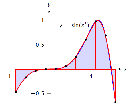
Figure \(\PageIndex{8}\): Approximating \(\int_{-\frac{\pi}4}^{\frac{\pi}2}\sin(x^3)\ dx\) in Example \(\PageIndex{6}\) with Simpson's Rule and 10 equally spaced intervals.

Recall that the actual value, accurate to 3 decimal places, is 0.460. Our approximation is within one 1/100\(^\text{th}\) of the correct value. The graph in Figure \(\PageIndex{8}\) shows how closely the parabolas match the shape of the graph.

Summary and Error Analysis

We summarize the key concepts of this section thus far in the following Key Idea.

Key Idea 9: Numerical Integration

Let \(f\) be a continuous function on \([a,b]\), let \(n\) be a positive integer, and let \(\Delta x = \frac{b-a}{n}\).

Set \(x_1=a\), \(x_2 = a+\ dx\), \(\ldots\), \(x_i = a+(i-1)\ dx\), \(x_{n+1}=b\).

Consider \(\int_a^b f(x)\ dx\).

Left Hand Rule: \(\int_a^b f(x)\ dx \approx \ dx\Big[f(x_1) + f(x_2) + \ldots + f(x_n)\big]\).

Right Hand Rule: \(\int_a^b f(x)\ dx \approx \ dx\Big[f(x_2) + f(x_3) + \ldots + f(x_{n+1})\big]\).

Trapezoidal Rule: \(\int_a^b f(x)\ dx \approx \frac{\ dx}2\Big[f(x_1) + 2f(x_2) + 2f(x_3) +\ldots + 2f(x_n)+ f(x_{n+1})\big]\).

Simpson's Rule: \(\int_a^b f(x)\ dx \approx \frac{\ dx}3\Big[f(x_1) + 4f(x_2) + 2f(x_3) +\ldots + 4f(x_n)+ f(x_{n+1})\big]\) (\(n\) even)}.

In our examples, we approximated the value of a definite integral using a given method then compared it to the "right" answer. This should have raised several questions in the reader's mind, such as:

1. How was the "right" answer computed?
2. If the right answer can be found, what is the point of approximating?
3. If there is value to approximating, how are we supposed to know if the approximation is any good?

These are good questions, and their answers are educational. In the examples, the right answer was never computed. Rather, an approximation accurate to a certain number of places after the decimal was given. In Example \(\PageIndex{1}\), we do not know the exact answer, but we know it starts with 0.7468. These more accurate approximations were computed using numerical integration but with more precision (i.e., more subintervals and the help of a computer).

Since the exact answer cannot be found, approximation still has its place. How are we to tell if the approximation is any good?

"Trial and error" provides one way. Using technology, make an approximation with, say, 10, 100, and 200 subintervals. This likely will not take much time at all, and a trend should emerge. If a trend does not emerge, try using yet more subintervals. Keep in mind that trial and error is never foolproof; you might stumble upon a problem in which a trend will not emerge.

A second method is to use Error Analysis. While the details are beyond the scope of this text, there are some formulas that give bounds for how good your approximation will be. For instance, the formula might state that the approximation is within 0.1 of the correct answer. If the approximation is 1.58, then one knows that the correct answer is between 1.48 and 1.68. By using lots of subintervals, one can get an approximation as accurate as one likes. Theorem \(\PageIndex{1}\) states what these bounds are.

Theorem \(\PageIndex{1}\): Error Bounds in the Trapezoidal and Simpson's Rules

1. Let \(E_T\) be the error in approximating \( \int_a^b f(x)\ dx\) using the Trapezoidal Rule.
   If \(f\) has a continuous 2\(^\text{nd}\) derivative on \([a,b]\) and \(M\) is any upper bound of \(\big|f"(x)\big|\) on \([a,b]\), then

$$ E_T \leq \frac{(b-a)^3}{12n^2}M.\]

2. Let \(E_S\) be the error in approximating \( \int_a^b f(x)\ dx\) using Simpson's Rule.
   If \(f\) has a continuous 4\(^\text{th}\) derivative on \([a,b]\) and \(M\) is any upper bound of \(\big|f\,^{(4)}\big|\) on \([a,b]\), then

$$E_S \leq \frac{(b-a)^5}{180n^4}M.\]

There are some key things to note about this theorem.

1. The larger the interval, the larger the error. This should make sense intuitively.
2. The error shrinks as more subintervals are used (i.e., as \(n\) gets larger).
3. The error in Simpson's Rule has a term relating to the 4\(^{\text{th}}\) derivative of \(f\). Consider a cubic polynomial: it's \(4^{\text{th}}\) derivative is 0. Therefore, the error in approximating the definite integral of a cubic polynomial with Simpson's Rule is 0 -- Simpson's Rule computes the exact answer!

We revisit Examples \(\PageIndex{3}\) and \(\PageIndex{5}\) and compute the error bounds using Theorem \(\PageIndex{1}\) in the following example.

Example \(\PageIndex{7}\): Computing error bounds

Find the error bounds when approximating \( \int_0^1 e^{-x^2}\ dx\) using the Trapezoidal Rule and 5 subintervals, and using Simpson's Rule with 4 subintervals.

Solution

Trapezoidal Rule with \(n=5\):

We start by computing the \(2^\text{nd}\) derivative of \(f(x) = e^{-x^2}\):

\[f"(x) = e^{-x^2}(4x^2-2).\]

Figure \(\PageIndex{8}\) shows a graph of \(f"(x)\) on \([0,1]\). It is clear that the largest value of \(f"\), in absolute value, is 2. Thus we let \(M=2\) and apply the error formula from Theorem \(\PageIndex{1}\).

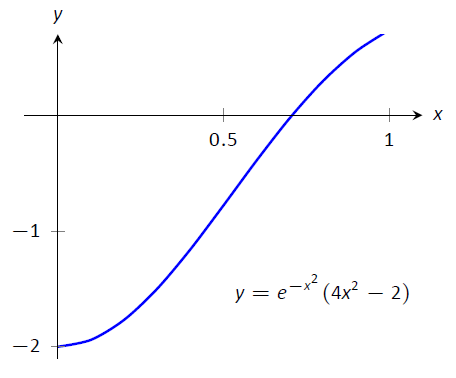
Figure \(\PageIndex{9}\): Graphing \(f"(x)\) in Example \(\PageIndex{7}\) to help establish error bounds.

$$E_T = \frac{(1-0)^3}{12\cdot 5^2}\cdot 2 = 0.00\overline{6}.\]

Our error estimation formula states that our approximation of 0.7445 found in Example \(\PageIndex{3}\) is within 0.0067 of the correct answer, hence we know that

$$0.7445-0.0067 = .7378 \leq \int_0^1e^{-x^2}\ dx \leq 0.7512 = 0.7445 + 0.0067.\]

We had earlier computed the exact answer, correct to 4 decimal places, to be 0.7468, affirming the validity of Theorem \(\PageIndex{1}\).

Simpson's Rule with \(n=4\):

We start by computing the \(4^\text{th}\) derivative of \(f(x) = e^{-x^2}\):

$$f\,^{(4)}(x) = e^{-x^2}(16x^4-48x^2+12).\]

Figure \(\PageIndex{9}\) shows a graph of \(f\,^{(4)}(x)\) on \([0,1]\). It is clear that the largest value of \(f\,^{(4)}\), in absolute value, is 12. Thus we let \(M=12\) and apply the error formula from Theorem \(\PageIndex{1}\).

$$E_s = \frac{(1-0)^5}{180\cdot 4^4}\cdot 12 = 0.00026.\]

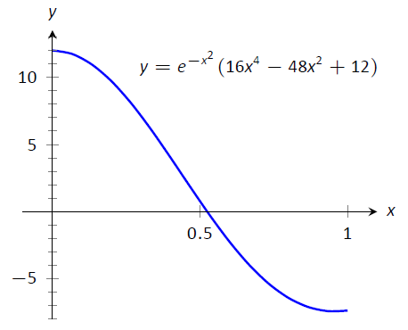
Figure \(\PageIndex{10}\): Graphing \(f\,^{(4)}(x)\) in Example \(\PageIndex{7}\) to help establish error bounds.

Our error estimation formula states that our approximation of \(0.7468\overline{3}\) found in Example \(\PageIndex{5}\) is within 0.00026 of the correct answer, hence we know that

$$0.74683-0.00026 = .74657 \leq \int_0^1e^{-x^2}\ dx \leq 0.74709 = 0.74683 + 0.00026.\]

Once again we affirm the validity of Theorem\(\PageIndex{1}\).

At the beginning of this section we mentioned two main situations where numerical integration was desirable. We have considered the case where an antiderivative of the integrand cannot be computed. We now investigate the situation where the integrand is not known. This is, in fact, the most widely used application of Numerical Integration methods. "Most of the time" we observe behavior but do not know "the" function that describes it. We instead collect data about the behavior and make approximations based off of this data. We demonstrate this in an example.

Example \(\PageIndex{8}\): Approximating distance traveled

One of the authors drove his daughter home from school while she recorded their speed every 30 seconds. The data is given in Table \(\PageIndex{5}\). Approximate the distance they traveled.

Solution

Recall that by integrating a speed function we get distance traveled. We have information about \(v(t)\); we will use Simpson's Rule to approximate \(\int_a^b v(t)\ dt.\)

The most difficult aspect of this problem is converting the given data into the form we need it to be in. The speed is measured in miles per hour, whereas the time is measured in 30 second increments.

Table \(\PageIndex{5}\): Speed data collected at 30 second intervals for Example \(\PageIndex{8}\).

0	0
1	25
2	22
3	19
4	39
5	0
6	43
7	59
8	54
9	51
10	43
11	35
12	40
13	43
14	30
15	0
16	0
17	28
18	40
19	42
20	40
21	39
22	40
23	23
24	0

We need to compute \(\ dx = (b-a)/n\). Clearly, \(n=24\). What are \(a\) and \(b\)? Since we start at time \(t=0\), we have that \(a=0\). The final recorded time came after 24 periods of 30 seconds, which is 12 minutes or 1/5 of an hour. Thus we have

$$\ dx = \frac{b-a}{n} = \frac{1/5-0}{24} = \frac1{120}; \quad \frac{\ dx}{3} = \frac{1}{360}.\]

Thus the distance traveled is approximately:

\[ \begin{align*} \int_0^{0.2}v(t)\ dt &\approx \frac{1}{360}\Big[f(x_1)+4f(x_2) + 2f(x_3) + \cdots + 4f(x_n)+f(x_{n+1})\Big]\\
&= \frac{1}{360}\Big[0+4\cdot25+2\cdot 22 + \cdots + 2\cdot40+4\cdot 23 + 0\Big]\\ &\approx 6.2167 \ \text{miles.}\end{align*}\]

We approximate the author drove 6.2 miles. (Because we are sure the reader wants to know, the author's odometer recorded the distance as about 6.05 miles.)

We started this chapter learning about antiderivatives and indefinite integrals. We then seemed to change focus by looking at areas between the graph of a function and the \(x\)-axis. We defined these areas as the definite integral of the function, using a notation very similar to the notation of the indefinite integral. The Fundamental Theorem of Calculus tied these two seemingly separate concepts together: we can find areas under a curve, i.e., we can evaluate a definite integral, using antiderivatives.

We ended the chapter by noting that antiderivatives are sometimes more than difficult to find: they are impossible. Therefore we developed numerical techniques that gave us good approximations of definite integrals.

We used the definite integral to compute areas, and also to compute displacements and distances traveled. There is far more we can do than that. In Chapter 7 we'll see more applications of the definite integral. Before that, in Chapter 6 we'll learn advanced techniques of integration, analogous to learning rules like the Product, Quotient and Chain Rules of differentiation.

Contributors and Attributions

• Gregory Hartman (Virginia Military Institute). Contributions were made by Troy Siemers and Dimplekumar Chalishajar of VMI and Brian Heinold of Mount Saint Mary's University. This content is copyrighted by a Creative Commons Attribution - Noncommercial (BY-NC) License. http://www.apexcalculus.com/

• Integrated by Justin Marshall.