
5.1: Maxima and Minima
- Page ID
- 455

\( \newcommand{\vecs}[1]{\overset { \scriptstyle \rightharpoonup} {\mathbf{#1}} } \)
\( \newcommand{\vecd}[1]{\overset{-\!-\!\rightharpoonup}{\vphantom{a}\smash {#1}}} \)
\( \newcommand{\dsum}{\displaystyle\sum\limits} \)
\( \newcommand{\dint}{\displaystyle\int\limits} \)
\( \newcommand{\dlim}{\displaystyle\lim\limits} \)
\( \newcommand{\id}{\mathrm{id}}\) \( \newcommand{\Span}{\mathrm{span}}\)
( \newcommand{\kernel}{\mathrm{null}\,}\) \( \newcommand{\range}{\mathrm{range}\,}\)
\( \newcommand{\RealPart}{\mathrm{Re}}\) \( \newcommand{\ImaginaryPart}{\mathrm{Im}}\)
\( \newcommand{\Argument}{\mathrm{Arg}}\) \( \newcommand{\norm}[1]{\| #1 \|}\)
\( \newcommand{\inner}[2]{\langle #1, #2 \rangle}\)
\( \newcommand{\Span}{\mathrm{span}}\)
\( \newcommand{\id}{\mathrm{id}}\)
\( \newcommand{\Span}{\mathrm{span}}\)
\( \newcommand{\kernel}{\mathrm{null}\,}\)
\( \newcommand{\range}{\mathrm{range}\,}\)
\( \newcommand{\RealPart}{\mathrm{Re}}\)
\( \newcommand{\ImaginaryPart}{\mathrm{Im}}\)
\( \newcommand{\Argument}{\mathrm{Arg}}\)
\( \newcommand{\norm}[1]{\| #1 \|}\)
\( \newcommand{\inner}[2]{\langle #1, #2 \rangle}\)
\( \newcommand{\Span}{\mathrm{span}}\) \( \newcommand{\AA}{\unicode[.8,0]{x212B}}\)
\( \newcommand{\vectorA}[1]{\vec{#1}} % arrow\)
\( \newcommand{\vectorAt}[1]{\vec{\text{#1}}} % arrow\)
\( \newcommand{\vectorB}[1]{\overset { \scriptstyle \rightharpoonup} {\mathbf{#1}} } \)
\( \newcommand{\vectorC}[1]{\textbf{#1}} \)
\( \newcommand{\vectorD}[1]{\overrightarrow{#1}} \)
\( \newcommand{\vectorDt}[1]{\overrightarrow{\text{#1}}} \)
\( \newcommand{\vectE}[1]{\overset{-\!-\!\rightharpoonup}{\vphantom{a}\smash{\mathbf {#1}}}} \)
\( \newcommand{\vecs}[1]{\overset { \scriptstyle \rightharpoonup} {\mathbf{#1}} } \)
\(\newcommand{\longvect}{\overrightarrow}\)
\( \newcommand{\vecd}[1]{\overset{-\!-\!\rightharpoonup}{\vphantom{a}\smash {#1}}} \)
\(\newcommand{\avec}{\mathbf a}\) \(\newcommand{\bvec}{\mathbf b}\) \(\newcommand{\cvec}{\mathbf c}\) \(\newcommand{\dvec}{\mathbf d}\) \(\newcommand{\dtil}{\widetilde{\mathbf d}}\) \(\newcommand{\evec}{\mathbf e}\) \(\newcommand{\fvec}{\mathbf f}\) \(\newcommand{\nvec}{\mathbf n}\) \(\newcommand{\pvec}{\mathbf p}\) \(\newcommand{\qvec}{\mathbf q}\) \(\newcommand{\svec}{\mathbf s}\) \(\newcommand{\tvec}{\mathbf t}\) \(\newcommand{\uvec}{\mathbf u}\) \(\newcommand{\vvec}{\mathbf v}\) \(\newcommand{\wvec}{\mathbf w}\) \(\newcommand{\xvec}{\mathbf x}\) \(\newcommand{\yvec}{\mathbf y}\) \(\newcommand{\zvec}{\mathbf z}\) \(\newcommand{\rvec}{\mathbf r}\) \(\newcommand{\mvec}{\mathbf m}\) \(\newcommand{\zerovec}{\mathbf 0}\) \(\newcommand{\onevec}{\mathbf 1}\) \(\newcommand{\real}{\mathbb R}\) \(\newcommand{\twovec}[2]{\left[\begin{array}{r}#1 \\ #2 \end{array}\right]}\) \(\newcommand{\ctwovec}[2]{\left[\begin{array}{c}#1 \\ #2 \end{array}\right]}\) \(\newcommand{\threevec}[3]{\left[\begin{array}{r}#1 \\ #2 \\ #3 \end{array}\right]}\) \(\newcommand{\cthreevec}[3]{\left[\begin{array}{c}#1 \\ #2 \\ #3 \end{array}\right]}\) \(\newcommand{\fourvec}[4]{\left[\begin{array}{r}#1 \\ #2 \\ #3 \\ #4 \end{array}\right]}\) \(\newcommand{\cfourvec}[4]{\left[\begin{array}{c}#1 \\ #2 \\ #3 \\ #4 \end{array}\right]}\) \(\newcommand{\fivevec}[5]{\left[\begin{array}{r}#1 \\ #2 \\ #3 \\ #4 \\ #5 \\ \end{array}\right]}\) \(\newcommand{\cfivevec}[5]{\left[\begin{array}{c}#1 \\ #2 \\ #3 \\ #4 \\ #5 \\ \end{array}\right]}\) \(\newcommand{\mattwo}[4]{\left[\begin{array}{rr}#1 \amp #2 \\ #3 \amp #4 \\ \end{array}\right]}\) \(\newcommand{\laspan}[1]{\text{Span}\{#1\}}\) \(\newcommand{\bcal}{\cal B}\) \(\newcommand{\ccal}{\cal C}\) \(\newcommand{\scal}{\cal S}\) \(\newcommand{\wcal}{\cal W}\) \(\newcommand{\ecal}{\cal E}\) \(\newcommand{\coords}[2]{\left\{#1\right\}_{#2}}\) \(\newcommand{\gray}[1]{\color{gray}{#1}}\) \(\newcommand{\lgray}[1]{\color{lightgray}{#1}}\) \(\newcommand{\rank}{\operatorname{rank}}\) \(\newcommand{\row}{\text{Row}}\) \(\newcommand{\col}{\text{Col}}\) \(\renewcommand{\row}{\text{Row}}\) \(\newcommand{\nul}{\text{Nul}}\) \(\newcommand{\var}{\text{Var}}\) \(\newcommand{\corr}{\text{corr}}\) \(\newcommand{\len}[1]{\left|#1\right|}\) \(\newcommand{\bbar}{\overline{\bvec}}\) \(\newcommand{\bhat}{\widehat{\bvec}}\) \(\newcommand{\bperp}{\bvec^\perp}\) \(\newcommand{\xhat}{\widehat{\xvec}}\) \(\newcommand{\vhat}{\widehat{\vvec}}\) \(\newcommand{\uhat}{\widehat{\uvec}}\) \(\newcommand{\what}{\widehat{\wvec}}\) \(\newcommand{\Sighat}{\widehat{\Sigma}}\) \(\newcommand{\lt}{<}\) \(\newcommand{\gt}{>}\) \(\newcommand{\amp}{&}\) \(\definecolor{fillinmathshade}{gray}{0.9}\)A local maximum point on a function is a point \((x,y)\) on the graph of the function whose \(y\) coordinate is larger than all other \(y\) coordinates on the graph at points "close to'' \((x,y)\). More precisely, \((x,f(x))\) is a local maximum if there is an interval \((a,b)\) with \(a < x < b\) and \(f(x)\ge f(z)\) for every \(z\) in \((a,b)\). Similarly, \((x,y)\) is a local minimum point if it has locally the smallest \(y\) coordinate. Again being more precise: \((x,f(x))\) is a local minimum if there is an interval \((a,b)\) with \(a < x < b\) and \(f(x)\le f(z)\) for every \(z\) in \((a,b)\). A local extremum is either a local minimum or a local maximum.
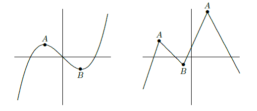
Local maximum and minimum points are quite distinctive on the graph of a function, and are therefore useful in understanding the shape of the graph. In many applied problems we want to find the largest or smallest value that a function achieves (for example, we might want to find the minimum cost at which some task can be performed) and so identifying maximum and minimum points will be useful for applied problems as well. Some examples of local maximum and minimum points are shown in figure 5.1.1.
If \((x,f(x))\) is a point where \(f(x)\) reaches a local maximum or minimum, and if the derivative of \(f\) exists at \(x\), then the graph has a tangent line and the tangent line must be horizontal. This is important enough to state as a theorem, though we will not prove it.
If \(f(x)\) has a local extremum at \(x=a\) and \(f\) is differentiable at \(a\), then \(f'(a)=0\).
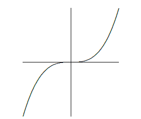
Thus, the only points at which a function can have a local maximum or minimum are points at which the derivative is zero, as in the left hand graph in figure 5.1.1, or the derivative is undefined, as in the right hand graph. Any value of \(x\) for which \(f'(x)\) is zero or undefined is called a critical value for \(f\). When looking for local maximum and minimum points, you are likely to make two sorts of mistakes: You may forget that a maximum or minimum can occur where the derivative does not exist, and so forget to check whether the derivative exists everywhere. You might also assume that any place that the derivative is zero is a local maximum or minimum point, but this is not true. A portion of the graph of \( f(x)=x^3\) is shown in figure 5.1.2. The derivative of \(f\) is \(f'(x)=3x^2\), and \(f'(0)=0\), but there is neither a maximum nor minimum at \((0,0)\).
Since the derivative is zero or undefined at both local maximum and local minimum points, we need a way to determine which, if either, actually occurs. The most elementary approach, but one that is often tedious or difficult, is to test directly whether the \(y\) coordinates "near'' the potential maximum or minimum are above or below the \(y\) coordinate at the point of interest. Of course, there are too many points "near'' the point to test, but a little thought shows we need only test two provided we know that \(f\) is continuous (recall that this means that the graph of \(f\) has no jumps or gaps).
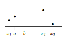
Suppose, for example, that we have identified three points at which \(f'\) is zero or nonexistent: \( (x_1,y_1)\), \( (x_2,y_2)\), \( (x_3,y_3)\), and \( x_1 < x_2 < x_3\) (see figure 5.1.3). Suppose that we compute the value of \(f(a)\) for \( x_1 < a < x_2\), and that \( f(a) < f(x_2)\). What can we say about the graph between \(a\) and \( x_2\); Could there be a point \( (b,f(b))\), \( a < b < x_2\) with \( f(b)>f(x_2)\); No: if there were, the graph would go up from \((a,f(a))\) to \((b,f(b))\) then down to \( (x_2,f(x_2))\) and somewhere in between would have a local maximum point. (This is not obvious; it is a result of the Extreme Value Theorem, theorem 6.1.2.) But at that local maximum point the derivative of \(f\) would be zero or nonexistent, yet we already know that the derivative is zero or nonexistent only at \( x_1\), \( x_2\), and \( x_3\).
The upshot is that one computation tells us that \( (x_2,f(x_2))\) has the largest \(y\) coordinate of any point on the graph near \( x_2\) and to the left of \( x_2\). We can perform the same test on the right. If we find that on both sides of \( x_2\) the values are smaller, then there must be a local maximum at \( (x_2,f(x_2))\); if we find that on both sides of \( x_2\) the values are larger, then there must be a local minimum at \( (x_2,f(x_2))\); if we find one of each, then there is neither a local maximum or minimum at \( x_2\).
It is not always easy to compute the value of a function at a particular point. The task is made easier by the availability of calculators and computers, but they have their own drawbacks---they do not always allow us to distinguish between values that are very close together. Nevertheless, because this method is conceptually simple and sometimes easy to perform, you should always consider it.
-2\sqrt{3}/9\) and \( f(1)=0>-2\sqrt{3}/9\), there must be a local minimum at \( x=\sqrt{3}/3\). For \( x=-\sqrt{3}/3\), we see that \( f(-\sqrt{3}/3)=2\sqrt{3}/9\). This time we can use \(x=0\) and \(x=-1\), and we find that \( f(-1)=f(0)=0 < 2\sqrt{3}/9\), so there must be a local maximum at \( x=-\sqrt{3}/3\).
Of course this example is made very simple by our choice of points to test, namely \(x=-1\), \(0\), \(1\). We could have used other values, say \(-5/4\), \(1/3\), and \(3/4\), but this would have made the calculations considerably more tedious.
We use \(\pi\) and \(2\pi\) to test the critical value \(x=5\pi/4\). The relevant values are \( f(5\pi/4)=-\sqrt2\), \( f(\pi)=-1>-\sqrt2\), \( f(2\pi)=1>-\sqrt2\), so there is a local minimum at \(x=5\pi/4\), \(5\pi/4\pm2\pi\), \(5\pi/4\pm4\pi\), etc. More succinctly, there are local minima at \(5\pi/4\pm 2k\pi\) for every integer \(k\).