6.5: Physical Applications of Integration

Learning Objectives

• Determine the mass of a one-dimensional object from its linear density function.
• Determine the mass of a two-dimensional circular object from its radial density function.
• Calculate the work done by a variable force acting along a line.
• Calculate the work done in pumping a liquid from one height to another.
• Find the hydrostatic force against a submerged vertical plate.

In this section, we examine some physical applications of integration. Let’s begin with a look at calculating mass from a density function. We then turn our attention to work, and close the section with a study of hydrostatic force.

Mass and Density

We can use integration to develop a formula for calculating mass based on a density function. First we consider a thin rod or wire. Orient the rod so it aligns with the \(x\)-axis, with the left end of the rod at \(x=a\) and the right end of the rod at \(x=b\) (Figure \(\PageIndex{1}\)). Note that although we depict the rod with some thickness in the figures, for mathematical purposes we assume the rod is thin enough to be treated as a one-dimensional object.

Figure \(\PageIndex{1}\): We can calculate the mass of a thin rod oriented along the \(x\)-axis by integrating its density function.

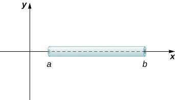
If the rod has constant density \(ρ\), given in terms of mass per unit length, then the mass of the rod is just the product of the density and the length of the rod: \((b−a)ρ\). If the density of the rod is not constant, however, the problem becomes a little more challenging. When the density of the rod varies from point to point, we use a linear density function, \(ρ(x)\), to denote the density of the rod at any point, \(x\). Let \(ρ(x)\) be an integrable linear density function. Now, for \(i=0,1,2,…,n\) let \(P={x_i}\) be a regular partition of the interval \([a,b]\), and for \(i=1,2,…,n\) choose an arbitrary point \(x^∗_i∈[x_{i−1},x_i]\). Figure \(\PageIndex{2}\) shows a representative segment of the rod.

Figure \(\PageIndex{2}\): A representative segment of the rod.

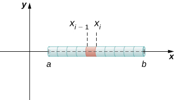
The mass \(m_i\) of the segment of the rod from \(x_{i−1}\) to \(x_i\) is approximated by

\[ \begin{align*} m_i ≈ρ(x^∗_i)(x_i−x_{i−1}) \\[4pt] =ρ(x^∗_i)Δx. \end{align*} \nonumber \]

Adding the masses of all the segments gives us an approximation for the mass of the entire rod:

\[ \begin{align*} m =\sum_{i=1}^nm_i \\[4pt] ≈\sum_{i=1}^nρ(x^∗_i)Δx. \end{align*} \nonumber \]

This is a Riemann sum. Taking the limit as \(n→∞\), we get an expression for the exact mass of the rod:

\[ \begin{align*} m =\lim_{n→∞}\sum_{i=1}^nρ(x^∗_i)Δx \\[4pt] =\int ^b_aρ(x)dx. \end{align*} \nonumber \]

We state this result in the following theorem.

Mass–Density Formula of a One-Dimensional Object

Given a thin rod oriented along the \(x\)-axis over the interval \([a,b]\), let \(ρ(x)\) denote a linear density function giving the density of the rod at a point \(x\) in the interval. Then the mass of the rod is given by

\[m=\int ^b_aρ(x)dx. \label{density1} \]

We apply this theorem in the next example.

Example \(\PageIndex{1}\): Calculating Mass from Linear Density

Consider a thin rod oriented on the \(x\)-axis over the interval \([π/2,π]\). If the density of the rod is given by \(ρ(x)=\sin x\), what is the mass of the rod?

Solution

Applying Equation \ref{density1} directly, we have

\[ \begin{align*} m =\int ^b_aρ(x)dx \nonumber \\[4pt] = \int ^π_{π/2}\sin x \,dx \nonumber \\[4pt] = −\cos x \Big|^π_{π/2} \nonumber \\[4pt] = 1. \nonumber \end{align*}\]

Exercise \(\PageIndex{1}\)

Consider a thin rod oriented on the \(x\)-axis over the interval \([1,3]\). If the density of the rod is given by \(ρ(x)=2x^2+3,\) what is the mass of the rod?

Hint

Use the process from the previous example.

Solution

\(70/3\)

We now extend this concept to find the mass of a two-dimensional disk of radius \(r\). As with the rod we looked at in the one-dimensional case, here we assume the disk is thin enough that, for mathematical purposes, we can treat it as a two-dimensional object. We assume the density is given in terms of mass per unit area (called area density), and further assume the density varies only along the disk’s radius (called radial density). We orient the disk in the \(xy-plane\), with the center at the origin. Then, the density of the disk can be treated as a function of \(x\), denoted \(ρ(x)\). We assume \(ρ(x)\) is integrable. Because density is a function of \(x\), we partition the interval from \([0,r]\) along the \(x\)-axis. For \(i=0,1,2,…,n\), let \(P={x_i}\) be a regular partition of the interval \([0,r]\), and for \(i=1,2,…,n\), choose an arbitrary point \(x^∗_i∈[x_{i−1},x_i]\). Now, use the partition to break up the disk into thin (two-dimensional) washers. A disk and a representative washer are depicted in the following figure.

Figure \(\PageIndex{3}\): (a) A thin disk in the xy-plane. (b) A representative washer.

We now approximate the density and area of the washer to calculate an approximate mass, \(m_i\). Note that the area of the washer is given by

\[ \begin{align*} A_i =π(x_i)^2−π(x_{i−1})^2 \\[4pt] =π[x^2_i−x^2_{i−1}] \\[4pt] =π(x_i+x_{i−1})(x_i−x_{i−1}) \\[4pt] =π(x_i+x_{i−1})Δx. \end{align*}\]

You may recall that we had an expression similar to this when we were computing volumes by shells. As we did there, we use \(x^∗_i≈(x_i+x_{i−1})/2\) to approximate the average radius of the washer. We obtain

\[A_i=π(x_i+x_{i−1})Δx≈2πx^∗_iΔx. \nonumber \]

Using \(ρ(x^∗_i)\) to approximate the density of the washer, we approximate the mass of the washer by

\[m_i≈2πx^∗_iρ(x^∗_i)Δx. \nonumber \]

Adding up the masses of the washers, we see the mass \(m\) of the entire disk is approximated by

\[m=\sum_{i=1}^nm_i≈\sum_{i=1}^n2πx^∗_iρ(x^∗_i)Δx. \nonumber \]

We again recognize this as a Riemann sum, and take the limit as \(n→∞.\) This gives us

\[ \begin{align*} m =\lim_{n→∞}\sum_{i=1}^n2πx^∗_iρ(x^∗_i)Δx \\[4pt] =\int ^r_02πxρ(x)dx. \end{align*}\]

We summarize these findings in the following theorem.

Mass–Density Formula of a Circular Object

Let \(ρ(x)\) be an integrable function representing the radial density of a disk of radius \(r\). Then the mass of the disk is given by

\[m=\int ^r_02πxρ(x)dx. \label{massEq1} \]

Example \(\PageIndex{2}\): Calculating Mass from Radial Density

Let \(ρ(x)=\sqrt{x}\) represent the radial density of a disk. Calculate the mass of a disk of radius 4.

Solution

Applying Equation \ref{massEq1}, we find

\[ \begin{align*} m =\int ^r_02πxρ(x)dx \nonumber \\[4pt] =\int ^4_02πx\sqrt{x}dx=2π\int ^4_0x^{3/2}dx \nonumber \\[4pt] =2π\dfrac{2}{5}x^{5/2}∣^4_0=\dfrac{4π}{5}[32] \nonumber \\[4pt] =\dfrac{128π}{5}.\nonumber \end{align*}\]

Exercise \(\PageIndex{2}\)

Let \(ρ(x)=3x+2\) represent the radial density of a disk. Calculate the mass of a disk of radius 2.

Hint

Use the process from the previous example.

Solution

\(24π\)

Work Done by a Force

We now consider work. In physics, work is related to force, which is often intuitively defined as a push or pull on an object. When a force moves an object, we say the force does work on the object. In other words, work can be thought of as the amount of energy it takes to move an object. According to physics, when we have a constant force, work can be expressed as the product of force and distance.

In the English system, the unit of force is the pound and the unit of distance is the foot, so work is given in foot-pounds. In the metric system, kilograms and meters are used. One newton is the force needed to accelerate \(1\) kilogram of mass at the rate of \(1\) m/sec². Thus, the most common unit of work is the newton-meter. This same unit is also called the joule. Both are defined as kilograms times meters squared over seconds squared \((kg⋅m^2/s^2).\)

When we have a constant force, things are pretty easy. It is rare, however, for a force to be constant. The work done to compress (or elongate) a spring, for example, varies depending on how far the spring has already been compressed (or stretched). We look at springs in more detail later in this section.

Suppose we have a variable force \(F(x)\) that moves an object in a positive direction along the \(x\)-axis from point \(a\) to point \(b\). To calculate the work done, we partition the interval \([a,b]\) and estimate the work done over each subinterval. So, for \(i=0,1,2,…,n\), let \(P={x_i}\) be a regular partition of the interval \([a,b]\), and for \(i=1,2,…,n\), choose an arbitrary point \(x^∗_i∈[x_{i−1},x_i]\). To calculate the work done to move an object from point \(x_{i−1}\) to point \(x_i\), we assume the force is roughly constant over the interval, and use \(F(x^∗_i)\) to approximate the force. The work done over the interval \([x_{i−1},x_i]\), then, is given by

\[W_i≈F(x^∗_i)(x_{i}−x_{i−1})=F(x^∗_i)Δx. \nonumber \]

Therefore, the work done over the interval \([a,b]\) is approximately

\[W=\sum_{i=1}^nW_i≈\sum_{i=1}^nF(x^∗_i)Δx. \nonumber \]

Taking the limit of this expression as \(n→∞\) gives us the exact value for work:

\[ \begin{align*} W =\lim_{n→∞}\sum_{i=1}^nF(x^∗_i)Δx \\[4pt] =\int ^b_aF(x)dx. \end{align*}\]

Thus, we can define work as follows.

Definition: Work

If a variable force \(F(x)\) moves an object in a positive direction along the \(x\)-axis from point \(a\) to point \(b\), then the work done on the object is

\[W=\int ^b_aF(x)dx. \label{work} \]

Note that if \(F\) is constant, the integral evaluates to \(F⋅(b−a)=F⋅d,\) which is the formula we stated at the beginning of this section.

Now let’s look at the specific example of the work done to compress or elongate a spring. Consider a block attached to a horizontal spring. The block moves back and forth as the spring stretches and compresses. Although in the real world we would have to account for the force of friction between the block and the surface on which it is resting, we ignore friction here and assume the block is resting on a frictionless surface. When the spring is at its natural length (at rest), the system is said to be at equilibrium. In this state, the spring is neither elongated nor compressed, and in this equilibrium position the block does not move until some force is introduced. We orient the system such that \(x=0\) corresponds to the equilibrium position (Figure \(\PageIndex{4}\)).

Figure \(\PageIndex{4}\): A block attached to a horizontal spring at equilibrium, compressed, and elongated.

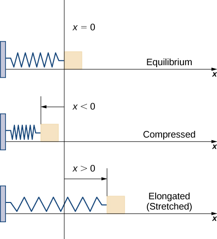
According to Hooke’s law, the force required to compress or stretch a spring from an equilibrium position is given by \(F(x)=kx\), for some constant \(k\). The value of k depends on the physical characteristics of the spring. The constant \(k\) is called the spring constant and is always positive. We can use this information to calculate the work done to compress or elongate a spring, as shown in the following example.

Example \(\PageIndex{3}\): The Work Required to Stretch or Compress a Spring

Suppose it takes a force of \(10\) N (in the negative direction) to compress a spring \(0.2\) m from the equilibrium position. How much work is done to stretch the spring \(0.5\) m from the equilibrium position?

Solution

First find the spring constant, \(k\). When \(x=−0.2\), we know \(F(x)=−10,\) so

\[ \begin{align*} F(x) =kx \\[4pt] −10 =k(−0.2) \\[4pt] k =50 \end{align*}\]

and \(F(x)=50x.\) Then, to calculate work, we integrate the force function, obtaining

\[\begin{align*} W = \int ^b_aF(x)dx \\[4pt] =\int ^{0.5}_050 x \,dx \\[4pt] =\left. 25x^2 \right|^{0.5}_0 \\[4pt] =6.25. \end{align*}\]

The work done to stretch the spring is \(6.25\) J.

Exercise \(\PageIndex{3}\)

Suppose it takes a force of \(8\) lb to stretch a spring \(6\) in. from the equilibrium position. How much work is done to stretch the spring \(1\) ft from the equilibrium position?

Hint

Use the process from the previous example. Be careful with units.

Solution

\(8\) ft-lb

Work Done in Pumping

Consider the work done to pump water (or some other liquid) out of a tank. Pumping problems are a little more complicated than spring problems because many of the calculations depend on the shape and size of the tank. In addition, instead of being concerned about the work done to move a single mass, we are looking at the work done to move a volume of water, and it takes more work to move the water from the bottom of the tank than it does to move the water from the top of the tank.

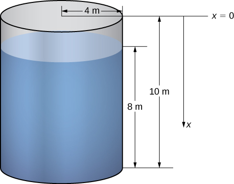
We examine the process in the context of a cylindrical tank, then look at a couple of examples using tanks of different shapes. Assume a cylindrical tank of radius \(4\) m and height \(10\) m is filled to a depth of 8 m. How much work does it take to pump all the water over the top edge of the tank?

The first thing we need to do is define a frame of reference. We let \(x\) represent the vertical distance below the top of the tank. That is, we orient the \(x\)-axis vertically, with the origin at the top of the tank and the downward direction being positive (Figure \(\PageIndex{5}\)).

Figure \(\PageIndex{5}\): How much work is needed to empty a tank partially filled with water?

Using this coordinate system, the water extends from \(x=2\) to \(x=10\). Therefore, we partition the interval \([2,10]\) and look at the work required to lift each individual “layer” of water. So, for \(i=0,1,2,…,n\), let \(P={x_i}\) be a regular partition of the interval \([2,10]\), and for \(i=1,2,…,n\), choose an arbitrary point \(x^∗_i∈[x_{i−1},x_i]\). Figure \(\PageIndex{6}\) shows a representative layer.

Figure \(\PageIndex{6}\): A representative layer of water.

In pumping problems, the force required to lift the water to the top of the tank is the force required to overcome gravity, so it is equal to the weight of the water. Given that the weight-density of water is \(9800 \, \text{N/m}^3\), or \(62.4\,\text{lb/ft}^3\), calculating the volume of each layer gives us the weight. In this case, we have

\[V=π(4)^2Δx=16πΔx. \nonumber \]

Then, the force needed to lift each layer is

\[F=9800⋅16πΔx=156,800πΔx. \nonumber \]

Note that this step becomes a little more difficult if we have a noncylindrical tank. We look at a noncylindrical tank in the next example.

We also need to know the distance the water must be lifted. Based on our choice of coordinate systems, we can use \(x^∗_i\) as an approximation of the distance the layer must be lifted. Then the work to lift the \(i^{\text{th}}\) layer of water \(W_i\) is approximately

\[W_i≈156,800πx^∗_iΔx. \nonumber \]

Adding the work for each layer, we see the approximate work to empty the tank is given by

\[ \begin{align*} W =\sum_{i=1}^nW_i \\[4pt] ≈\sum_{i=1}^n156,800πx^∗_iΔx.\end{align*}\]

This is a Riemann sum, so taking the limit as \(n→∞,\) we get

\[ \begin{align*} W =\lim_{n→∞}\sum^n_{i=1}156,800πx^∗_iΔx \\[4pt] = 156,800π\int ^{10}_2xdx \\[4pt] =156,800π \left( \dfrac{x^2}{2}\right)\bigg|^{10}_2=7,526,400π≈23,644,883. \end{align*}\]

The work required to empty the tank is approximately 23,650,000 J.

For pumping problems, the calculations vary depending on the shape of the tank or container. The following problem-solving strategy lays out a step-by-step process for solving pumping problems.

Problem-Solving Strategy: Solving Pumping Problems

1. Sketch a picture of the tank and select an appropriate frame of reference.
2. Calculate the volume of a representative layer of water.
3. Multiply the volume by the weight-density of water to get the force.
4. Calculate the distance the layer of water must be lifted.
5. Multiply the force and distance to get an estimate of the work needed to lift the layer of water.
6. Sum the work required to lift all the layers. This expression is an estimate of the work required to pump out the desired amount of water, and it is in the form of a Riemann sum.
7. Take the limit as \(n→∞\) and evaluate the resulting integral to get the exact work required to pump out the desired amount of water.

We now apply this problem-solving strategy in an example with a noncylindrical tank.

Example \(\PageIndex{4}\): A Pumping Problem with a Noncylindrical Tank

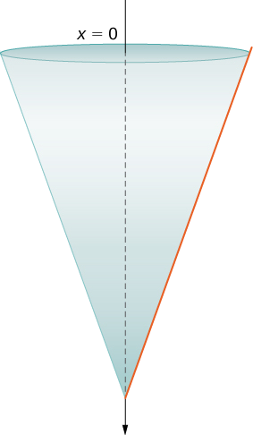
Assume a tank in the shape of an inverted cone, with height \(12\) ft and base radius \(4\) ft. The tank is full to start with, and water is pumped over the upper edge of the tank until the height of the water remaining in the tank is \(4\) ft. How much work is required to pump out that amount of water?

Solution

The tank is depicted in Figure \(\PageIndex{7}\). As we did in the example with the cylindrical tank, we orient the \(x\)-axis vertically, with the origin at the top of the tank and the downward direction being positive (step 1).

Figure \(\PageIndex{7}\): A water tank in the shape of an inverted cone.

The tank starts out full and ends with \(4\) ft of water left, so, based on our chosen frame of reference, we need to partition the interval \([0,8]\). Then, for \(i=0,1,2,…,n\), let \(P={x_i}\) be a regular partition of the interval \([0,8]\), and for \(i=1,2,…,n\), choose an arbitrary point \(x^∗_i∈[x_{i−1},x_i]\). We can approximate the volume of a layer by using a disk, then use similar triangles to find the radius of the disk (Figure \(\PageIndex{8}\)).

Figure \(\PageIndex{8}\): Using similar triangles to express the radius of a disk of water.

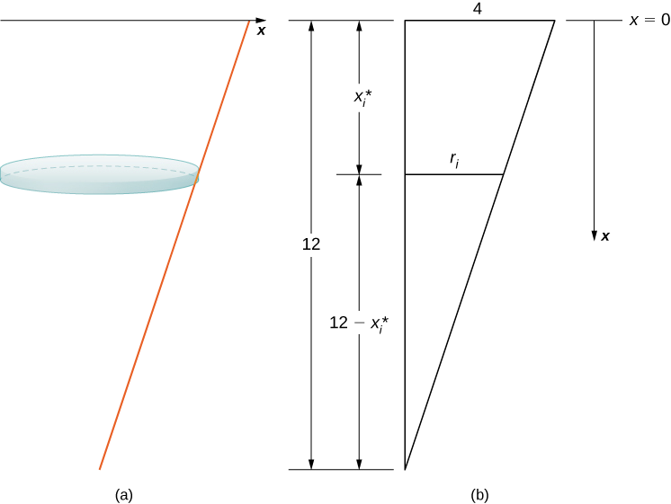
From properties of similar triangles, we have

\[ \begin{align*} \dfrac{r_i}{12−x^∗_i} =\dfrac{4}{12} \tag{step 1} =\dfrac{1}{3} \\[4pt] 3r_i =12−x^∗_i \\[4pt] r_i =\dfrac{12−x^∗_i}{3} \\[4pt] =4−\dfrac{x^∗_i}{3}. \end{align*} \]

Then the volume of the disk is

\[V_i=π \left(4−\dfrac{x^∗_i}{3}\right)^2\,Δx. \tag{step 2} \]

The weight-density of water is \(62.4\)lb/ft³, so the force needed to lift each layer is approximately

\[F_i≈62.4π\left(4−\dfrac{x^∗_i}{3}\right)^2\,Δx \tag{step 3} \]

Based on the diagram, the distance the water must be lifted is approximately \(x^∗_i\) feet (step 4), so the approximate work needed to lift the layer is

\[W_i≈62.4πx^∗_i\left(4−\dfrac{x^∗_i}{3}\right)^2\,Δx. \tag{step 5} \]

Summing the work required to lift all the layers, we get an approximate value of the total work:

\[W=\sum_{i=1}^nW_i≈\sum_{i=1}^n62.4πx^∗_i \left(4−\dfrac{x^∗_i}{3}\right)^2\,Δx. \tag{step 6} \]

Taking the limit as \(n→∞,\) we obtain

\[ \begin{align*} W =\lim_{n→∞}\sum^n_{i=1}62.4πx^∗_i(4−\dfrac{x^∗_i}{3})^2Δx \\[4pt] = \int ^8_062.4πx \left(4−\dfrac{x}{3}\right)^2dx \\[4pt] = 62.4π\int ^8_0x \left(16−\dfrac{8x}{3}+\dfrac{x^2}{9}\right)\,dx=62.4π\int ^8_0 \left(16x−\dfrac{8x^2}{3}+\dfrac{x^3}{9}\right)\,dx \\[4pt] =62.4π\left[8x^2−\dfrac{8x^3}{9}+\dfrac{x^4}{36}\right]\bigg|^8_0=10,649.6π≈33,456.7. \end{align*}\]

It takes approximately \(33,450\) ft-lb of work to empty the tank to the desired level.

Exercise \(\PageIndex{4}\)

A tank is in the shape of an inverted cone, with height \(10\) ft and base radius 6 ft. The tank is filled to a depth of 8 ft to start with, and water is pumped over the upper edge of the tank until 3 ft of water remain in the tank. How much work is required to pump out that amount of water?

Hint

Use the process from the previous example.

Solution

Approximately \(43,255.2\) ft-lb

Hydrostatic Force and Pressure

In this last section, we look at the force and pressure exerted on an object submerged in a liquid. In the English system, force is measured in pounds. In the metric system, it is measured in newtons. Pressure is force per unit area, so in the English system we have pounds per square foot (or, perhaps more commonly, pounds per square inch, denoted psi). In the metric system we have newtons per square meter, also called pascals.

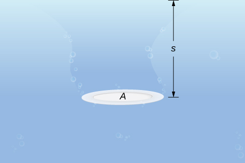
Let’s begin with the simple case of a plate of area \(A\) submerged horizontally in water at a depth s (Figure \(\PageIndex{9}\)). Then, the force exerted on the plate is simply the weight of the water above it, which is given by \(F=ρAs\), where \(ρ\) is the weight density of water (weight per unit volume). To find the hydrostatic pressure—that is, the pressure exerted by water on a submerged object—we divide the force by the area. So the pressure is \(p=F/A=ρs\).

Figure \(\PageIndex{9}\): A plate submerged horizontally in water.

By Pascal’s principle, the pressure at a given depth is the same in all directions, so it does not matter if the plate is submerged horizontally or vertically. So, as long as we know the depth, we know the pressure. We can apply Pascal’s principle to find the force exerted on surfaces, such as dams, that are oriented vertically. We cannot apply the formula \(F=ρAs\) directly, because the depth varies from point to point on a vertically oriented surface. So, as we have done many times before, we form a partition, a Riemann sum, and, ultimately, a definite integral to calculate the force.

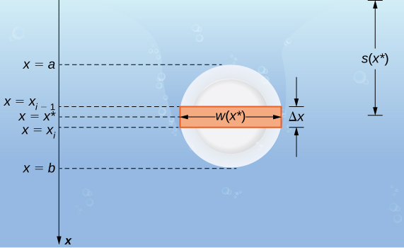
Suppose a thin plate is submerged in water. We choose our frame of reference such that the \(x\)-axis is oriented vertically, with the downward direction being positive, and point \(x=0\) corresponding to a logical reference point. Let \(s(x)\) denote the depth at point x. Note we often let \(x=0\) correspond to the surface of the water. In this case, depth at any point is simply given by \(s(x)=x\). However, in some cases we may want to select a different reference point for \(x=0\), so we proceed with the development in the more general case. Last, let \(w(x)\) denote the width of the plate at the point \(x\).

Assume the top edge of the plate is at point \(x=a\) and the bottom edge of the plate is at point \(x=b\). Then, for \(i=0,1,2,…,n\), let \(P={x_i}\) be a regular partition of the interval \([a,b]\), and for \(i=1,2,…,n\), choose an arbitrary point \(x^∗_i∈[x_{i−1},x_i]\). The partition divides the plate into several thin, rectangular strips (Figure \(\PageIndex{10}\)).

Figure \(\PageIndex{10}\): A thin plate submerged vertically in water.

Let’s now estimate the force on a representative strip. If the strip is thin enough, we can treat it as if it is at a constant depth, \(s(x^∗_i)\). We then have

\[F_i=ρAs=ρ[w(x^∗_i)Δx]s(x^∗_i). \nonumber \]

Adding the forces, we get an estimate for the force on the plate:

\[F≈\sum_{i=1}^nF_i=\sum_{i=1}^nρ[w(x^∗_i)Δx]s(x^∗_i). \nonumber \]

This is a Riemann sum, so taking the limit gives us the exact force. We obtain

\[F=\lim_{n→∞}\sum_{i=1}^nρ[w(x^∗_i)Δx]s(x^∗_i)=\int ^b_aρw(x)s(x)dx. \label{eqHydrostatic} \]

Evaluating this integral gives us the force on the plate. We summarize this in the following problem-solving strategy.

Problem-Solving Strategy: Finding Hydrostatic Force

1. Sketch a picture and select an appropriate frame of reference. (Note that if we select a frame of reference other than the one used earlier, we may have to adjust Equation \ref{eqHydrostatic} accordingly.)
2. Determine the depth and width functions, \(s(x)\) and \(w(x).\)
3. Determine the weight-density of whatever liquid with which you are working. The weight-density of water is \(62.4 \,\text{lb/ft}^3\), or \(9800 \,\text{N/m}^3\).
4. Use the equation to calculate the total force.

Example \(\PageIndex{5}\): Finding Hydrostatic Force

A water trough 15 ft long has ends shaped like inverted isosceles triangles, with base 8 ft and height 3 ft. Find the force on one end of the trough if the trough is full of water.

Solution

Figure \(\PageIndex{11}\) shows the trough and a more detailed view of one end.

Figure \(\PageIndex{11}\): (a) A water trough with a triangular cross-section. (b) Dimensions of one end of the water trough.

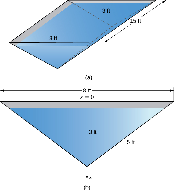
Select a frame of reference with the \(x\)-axis oriented vertically and the downward direction being positive. Select the top of the trough as the point corresponding to \(x=0\) (step 1). The depth function, then, is \(s(x)=x\). Using similar triangles, we see that \(w(x)=8−(8/3)x\) (step 2). Now, the weight density of water is \(62.4 \,\text{lb/ft}^3\) (step 3), so applying Equation \ref{eqHydrostatic}, we obtain

\[ \begin{align*} F =\int ^b_aρw(x)s(x)dx \\[4pt] = \int ^3_062.4 \left(8−\dfrac{8}{3}x\right) x \,dx=62.4\int ^3_0 \left(8x−\dfrac{8}{3}x^2 \right)dx \\[4pt] = \left.62.4 \left[4x^2−\dfrac{8}{9}x^3\right]\right|^3_0=748.8. \end{align*}\]

The water exerts a force of 748.8 lb on the end of the trough (step 4).

Exercise \(\PageIndex{5}\)

A water trough 12 m long has ends shaped like inverted isosceles triangles, with base 6 m and height 4 m. Find the force on one end of the trough if the trough is full of water.

Hint

Follow the problem-solving strategy and the process from the previous example.

Solution

\(156,800\) N

Example \(\PageIndex{6}\): Finding Hydrostatic Force

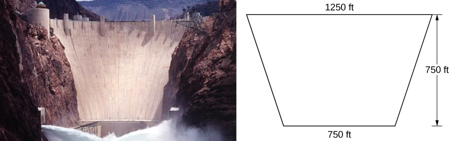
We now return our attention to the Hoover Dam, mentioned at the beginning of this chapter. The actual dam is arched, rather than flat, but we are going to make some simplifying assumptions to help us with the calculations. Assume the face of the Hoover Dam is shaped like an isosceles trapezoid with lower base 750 ft, upper base 1250 ft, and height 750 ft (see the following figure).

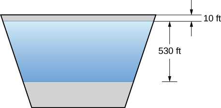
When the reservoir is full, Lake Mead’s maximum depth is about 530 ft, and the surface of the lake is about 10 ft below the top of the dam (see the following figure).

Figure \(\PageIndex{12}\): A simplified model of the Hoover Dam with assumed dimensions.

1. Find the force on the face of the dam when the reservoir is full.
2. The southwest United States has been experiencing a drought, and the surface of Lake Mead is about 125 ft below where it would be if the reservoir were full. What is the force on the face of the dam under these circumstances?

Solution:

a.

We begin by establishing a frame of reference. As usual, we choose to orient the \(x\)-axis vertically, with the downward direction being positive. This time, however, we are going to let \(x=0\) represent the top of the dam, rather than the surface of the water. When the reservoir is full, the surface of the water is \(10\) ft below the top of the dam, so \(s(x)=x−10\) (see the following figure).

Figure \(\PageIndex{13}\): We first choose a frame of reference.

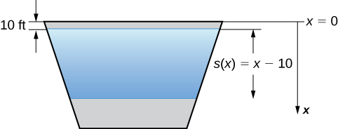
To find the width function, we again turn to similar triangles as shown in the figure below.

Figure \(\PageIndex{14}\): We use similar triangles to determine a function for the width of the dam. (a) Assumed dimensions of the dam; (b) highlighting the similar triangles.

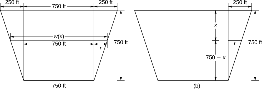
From the figure, we see that \(w(x)=750+2r\). Using properties of similar triangles, we get \(r=250−(1/3)x\). Thus,

\[w(x)=1250−\dfrac{2}{3}x \tag{step 2} \]

Using a weight-density of \(62.4\)lb/ft³ (step 3) and applying Equation \ref{eqHydrostatic}, we get

\[\begin{align*} F =\int^b_a ρw(x)s(x)\,dx \\[4pt]
=\int ^{540}_{10}62.4 \left(1250−\dfrac{2}{3}x\right)(x−10)\,dx \\[4pt]
=62.4\int ^{540}_{10}−\dfrac{2}{3}[x^2−1885x+18750]\,dx \\[4pt]
=−62.4\left(\dfrac{2}{3}\right)\left[\dfrac{x^3}{3}−\dfrac{1885x^2}{2}+18750x\right]\bigg|^{540}_{10}≈8,832,245,000 \,\text{lb}=4,416,122.5\,\text{t}. \end{align*}\]

Note the change from pounds to tons (\(2000\)lb = \(1\) ton) (step 4). This changes our depth function, \(s(x)\), and our limits of integration. We have \(s(x)=x−135\). The lower limit of integration is 135. The upper limit remains \(540\). Evaluating the integral, we get

\[\begin{align*} F =\int^b_aρw(x)s(x)\,dx \\[4pt]
=\int ^{540}_{135}62.4 \left(1250−\dfrac{2}{3}x\right)(x−135)\,dx \\[4pt]
=−62.4(\dfrac{2}{3})\int ^{540}_{135}(x−1875)(x−135)\,dx=−62.4\left(\dfrac{2}{3}\right)\int ^{540}_{135}(x^2−2010x+253125)\,dx \\[4pt]
=−62.4\left(\dfrac{2}{3}\right)\left[\dfrac{x^3}{3}−1005x^2+253125x\right]\bigg|^{540}_{135}≈5,015,230,000\,\text{lb}=2,507,615\,\text{t}. \end{align*}\]

Exercise \(\PageIndex{6}\)

When the reservoir is at its average level, the surface of the water is about 50 ft below where it would be if the reservoir were full. What is the force on the face of the dam under these circumstances?

Hint

Change the depth function, \(s(x),\) and the limits of integration.

Solution

Approximately 7,164,520,000 lb or 3,582,260 t

Key Concepts

• Several physical applications of the definite integral are common in engineering and physics.
• Definite integrals can be used to determine the mass of an object if its density function is known.
• Work can also be calculated from integrating a force function, or when counteracting the force of gravity, as in a pumping problem.
• Definite integrals can also be used to calculate the force exerted on an object submerged in a liquid.

Key Equations

• Mass of a one-dimensional object

\( \displaystyle m=\int ^b_aρ(x)dx\)

• Mass of a circular object

\(\displaystyle m=\int ^r_02πxρ(x)dx\)

• Work done on an object

\(\displaystyle W=\int ^b_aF(x)dx\)

• Hydrostatic force on a plate

\(\displaystyle F=\int ^b_aρw(x)s(x)dx\)

Glossary

density function

a density function describes how mass is distributed throughout an object; it can be a linear density, expressed in terms of mass per unit length; an area density, expressed in terms of mass per unit area; or a volume density, expressed in terms of mass per unit volume; weight-density is also used to describe weight (rather than mass) per unit volume

Hooke’s law

this law states that the force required to compress (or elongate) a spring is proportional to the distance the spring has been compressed (or stretched) from equilibrium; in other words, \(F=kx\), where \(k\) is a constant

hydrostatic pressure

the pressure exerted by water on a submerged object

work

the amount of energy it takes to move an object; in physics, when a force is constant, work is expressed as the product of force and distance