2.4: Directional Derivatives and the Gradient

For a function $z = f (x, y)$, we learned that the partial derivatives $\dfrac{∂f}{∂x}\text{ and} \dfrac{∂f}{∂y}$ represent the (instantaneous) rate of change of $f$ in the positive $x$ and $y$ directions, respectively. What about other directions? It turns out that we can find the rate of change in any direction using a more general type of derivative called a directional derivative.

Definition 2.5: directional derivative

Let $f (x, y)$ be a real-valued function with domain $D$ in $\mathbb{R}^2$, and let $(a,b)$ be a point in $D$. Let $\textbf{v}$ be a unit vector in $\mathbb{R}^2$. Then the directional derivative of $\textbf{f}$ at $\mathbf{(a,b)}$ in the direction of $\mathbf{v}$, denoted by $D_v f(a,b)$, is defined as

$$D_v f(a,b)=\lim \limits_{h \to 0}\dfrac{f((a,b)+h\textbf{v})-f(a,b)}{h}\label{Eq2.8}$$

Notice in the definition that we seem to be treating the point $(a,b)$ as a vector, since we are adding the vector $h\textbf{v}$ to it. But this is just the usual idea of identifying vectors with their terminal points, which the reader should be used to by now. If we were to write the vector $\textbf{v}$ as $\textbf{v} = (v_1 ,v_2)$, then

$$D_v f (a,b)=\lim \limits_{h \to 0}\dfrac{f (a+ hv_1 ,b + hv_2)− f (a,b)}{h}\label{Eq2.9}$$

From this we can immediately recognize that the partial derivatives $\dfrac{∂f}{∂x}\text{ and} \dfrac{∂f}{∂y}$ are special cases of the directional derivative with $\textbf{v} = \textbf{i} = (1,0)\text{ and } \textbf{v} = \textbf{j} = (0,1)$, respectively. That is, $\dfrac{∂f}{∂x} = D_i f\text{ and } \dfrac{∂f}{∂y} = D_j f$. Since there are many vectors with the same direction, we use a unit vector in the definition, as that represents a “standard” vector for a given direction.

If $f (x, y)$ has continuous partial derivatives $\dfrac{∂f}{∂x}\text{ and }\dfrac{∂f}{∂y}$ (which will always be the case in this text), then there is a simple formula for the directional derivative:

Theorem 2.2

Let $f (x, y)$ be a real-valued function with domain $D$ in $\mathbb{R}^2$ such that the partial derivatives $\dfrac{∂f}{∂x}\text{ and }\dfrac{∂f}{∂y}$ exist and are continuous in $D$. Let $(a,b)$ be a point in $D$, and let $\textbf{v} = (v_1 ,v_2)$ be a unit vector in $\mathbb{R}^2$. Then

$$D_v f (a,b) = v_1 \dfrac{∂f}{∂x} (a,b)+ v_2 \dfrac{∂f}{∂y} (a,b)\label{Eq2.10}$$

Proof: Note that if $\textbf{v} = \textbf{i}$ = (1,0) then the above formula reduces to $D_v f (a,b) = \dfrac{∂f}{∂x} (a,b)$, which we know is true since $D_i f = \dfrac{∂f}{∂x}$, as we noted earlier. Similarly, for $\textbf{v} = \textbf{j} = (0,1)$ the formula reduces to $D_v f (a,b) = \dfrac{∂f}{∂y} (a,b)$, which is true since $D_j f = \dfrac{∂f}{∂y}$. So since $\textbf{i} = (1,0)\text{ and }\textbf{j} = (0,1)$ are the only unit vectors in $\mathbb{R}^2$ with a zero component, then we need only show the formula holds for unit vectors $\textbf{v} = (v_1 ,v_2)\text{ with }v_1 \neq 0 \text{ and }v_2 \neq 0$. So fix such a vector $\textbf{v}$ and fix a number $h \neq 0$.

Then

$$f (a+ hv_1 ,b + hv_2)− f (a,b) = f (a+ hv_1 ,b + hv_2)− f (a+ hv_1 ,b)+ f (a+ hv_1 ,b)− f (a,b)\label{Eq2.11}$$

Since $h \neq 0 \text{ and }v_2 \neq 0$, then $hv_2 \neq 0$ and thus any number $c$ between $b \text{ and }b + hv_2$ can be written as $c = b+\alpha hv_2$ for some number $0 < \alpha < 1$. So since the function $f (a+hv_1 , y)$ is a realvalued function of $y$ (since $a + hv_1$ is a fixed number), then the Mean Value Theorem from single-variable calculus can be applied to the function $g(y) = f (a + hv_1 , y)$ on the interval $[b,b + hv_2]$ (or $[b + hv_2 ,b]$ if one of $h \text{ or }v_2$ is negative) to find a number $0 < \alpha < 1$ such that

$$\nonumber \dfrac{∂f}{∂y} (a+ hv_1 ,b +\alpha hv_2) = g ′ (b +\alpha hv_2)=\dfrac{g(b + hv_2)− g(b)}{b + hv_2 − b}=\dfrac{f (a+ hv_1 ,b + hv_2)− f (a+ hv_1 ,b)}{hv_2}$$

and so

$$\nonumber f (a+ hv_1 ,b + hv_2)− f (a+ hv_1 ,b) = hv_2 \dfrac{∂f}{∂y} (a+ hv_1 ,b +\alpha hv_2) .$$

By a similar argument, there exists a number $0 < \beta < 1$ such that

$$\nonumber f (a+ hv_1 ,b)− f (a,b) = hv_1 \dfrac{∂f}{∂x} (a+\beta hv_1 ,b) .$$

Thus, by Equation $\ref{Eq2.11}$, we have

$$\nonumber \begin{align} \dfrac{f (a+ hv_1 ,b + hv_2)− f (a,b)}{h}&=\dfrac{hv_2 \dfrac{∂f}{∂y} (a+ hv_1 ,b +\alpha hv_2)+ hv_1 \dfrac{∂f}{∂x} (a+\beta hv_1 ,b)}{h} \\[4pt] \nonumber &=v_2 \dfrac{∂f}{∂y} (a+ hv_1 ,b +\alpha hv_2)+ v_1 \dfrac{∂f}{∂x} (a+\beta hv_1 ,b)\end{align}$$

so by Equation $\ref{Eq2.9}$ we have

$$\nonumber \begin{align} D_v f (a,b)&=\lim \limits_{h \to 0}\dfrac{f (a+ hv_1 ,b + hv_2)− f (a,b)}{h} \\[4pt] \nonumber &=\lim \limits_{h \to 0}\left [v_2 \dfrac{∂f}{∂y} (a+ hv_1 ,b +\alpha hv_2)+ v_1 \dfrac{∂f}{∂x} (a+\beta hv_1 ,b)\right ] \\[4pt] \nonumber &= v_2 \dfrac{∂f}{∂y} (a,b)+ v_1 \dfrac{∂f}{∂x} (a,b) \text{ by the continuity of } \dfrac{∂f}{∂x} \text{ and } \dfrac{∂f}{∂y}\text{, so} \\[4pt] \nonumber D_v f (a,b) &= v_1 \dfrac{∂f}{∂x} (a,b)+ v_2 \dfrac{∂f}{∂y} (a,b) \end{align}$$

$$\nonumber \text{after reversing the order of summation.}\tag{\(\textbf{QED}\)}$$

Note that $D_v f (a,b) = v \cdot \left (\dfrac{∂f}{∂x} (a,b), \dfrac{∂f}{∂y} (a,b) \right )$. The second vector has a special name:

Definition 2.6

For a real-valued function $f (x, y)$, the gradient of $f$, denoted by $\nabla f$, is the vector

$$\nabla f =\left ( \dfrac{∂f}{∂x} , \dfrac{∂f}{∂y} \right ) \label{Eq2.12}$$

in $\mathbb{R}^2$. For a real-valued function $f (x, y, z)$, the gradient is the vector

$$\nabla f = \left ( \dfrac{∂f}{∂x} , \dfrac{∂f}{∂y} , \dfrac{∂f}{∂z}\right ) \label{Eq2.13}$$

in $\mathbb{R}^ 3$. The symbol $\nabla$ is pronounced “del”.

Corollary 2.3

$$\nonumber D_v f = \textbf{v} \cdot \nabla f$$

Example 2.15

Find the directional derivative of $f (x, y) = x y^2 + x^3 y$ at the point (1,2) in the direction of $\textbf{v} = \left ( \dfrac{1}{\sqrt{2}},\dfrac{1}{\sqrt{2}}\right )$.

Solution

We see that $\nabla f = (y^2 +3x^2 y,2x y+ x^3 )$, so

$$\nonumber D_v f (1,2) = \textbf{v}\cdot \nabla f (1,2) = \left ( \dfrac{1}{\sqrt{2}},\dfrac{1}{\sqrt{2}}\right ) \cdot (2^2 +3(1)^2 (2),2(1)(2)+1^3 ) = \dfrac{15}{\sqrt{2}}$$

A real-valued function $z = f (x, y)$ whose partial derivatives $\dfrac{∂f}{∂x}\text{ and }\dfrac{∂f}{∂y}$ exist and are continuous is called continuously differentiable. Assume that $f (x, y)$ is such a function and that $\nabla f \neq \textbf{0}$. Let $c$ be a real number in the range of $f$ and let $\textbf{v}$ be a unit vector in $\mathbb{R}^2$ which is tangent to the level curve $f (x, y) = c$ (see Figure 2.4.1).

Figure 2.4.1

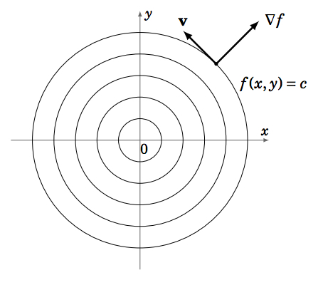
The value of $f (x, y)$ is constant along a level curve, so since $\textbf{v}$ is a tangent vector to this curve, then the rate of change of $f$ in the direction of $\textbf{v}$ is 0, i.e. $D_v f = 0$. But we know that $D_v f = \textbf{v} \cdot \nabla f = \left\lVert \textbf{v} \right\rVert \left\lVert \nabla f \right\rVert \cos \theta$, where $\theta$ is the angle between $\textbf{v} \text{ and }\nabla f$. So since $\left\lVert \textbf{v} \right\rVert = 1 \text{ then }D_v f = \left\lVert \nabla f \right\rVert \cos \theta$. So since $\nabla f \neq \textbf{0}\text{ then }D_v f = 0 ⇒ \cos \theta = 0 ⇒ \theta = 90^\circ$. In other words, $\nabla f \perp \textbf{v}$, which means that $\nabla f$ is normal to the level curve.

In general, for any unit vector $\textbf{v}$ in $\mathbb{R}^2$, we still have $D_v f = \left\lVert \nabla f \right\rVert \cos \theta \text{, where }\theta$ is the angle between $\textbf{v} \text{ and }\nabla f$. At a fixed point $(x, y)$ the length $\left\lVert \nabla f \right\rVert$ is fixed, and the value of $D_v f$ then varies as $\theta$ varies. The largest value that $D_v f$ can take is when $\cos \theta = 1 (\theta = 0^\circ )$, while the smallest value occurs when $\cos \theta = −1 (\theta = 180^\circ )$. In other words, the value of the function $f$ increases the fastest in the direction of $\nabla f$ (since $\theta = 0^\circ$ in that case), and the value of $f$ decreases the fastest in the direction of $−\nabla f$ (since $\theta = 180^\circ$ in that case). We have thus proved the following theorem:

Theorem 2.4

Let $f (x, y)$ be a continuously differentiable real-valued function, with $\nabla f \neq 0$. Then:

1. The gradient $\nabla f$ is normal to any level curve $f (x, y) = c$.
2. The value of $f (x, y)$ increases the fastest in the direction of $\nabla f$.
3. The value of $f (x, y)$ decreases the fastest in the direction of $−\nabla f$.

Example 2.16

In which direction does the function $f (x, y) = x y^2 + x^3 y$ increase the fastest from the point (1,2)? In which direction does it decrease the fastest?

Solution

Since $\nabla f = (y^2 + 3x^2 y,2xy + x^3 )$, then $\nabla f (1,2) = (10,5) \neq \textbf{0}$. A unit vector in that direction is $\textbf{v} = \dfrac{\nabla f}{\left\lVert \nabla f \right\rVert} = \left (\dfrac{2}{\sqrt{5}} ,\dfrac{1}{\sqrt{5}}\right )$. Thus, $f$ increases the fastest in the direction of $\left (\dfrac{2}{\sqrt{5}} ,\dfrac{1}{\sqrt{5}}\right )$ and decreases the fastest in the direction of $\left (\dfrac{−2}{\sqrt{5}},\dfrac{−1}{\sqrt{5}}\right )$.

Though we proved Theorem 2.4 for functions of two variables, a similar argument can be used to show that it also applies to functions of three or more variables. Likewise, the directional derivative in the three-dimensional case can also be defined by the formula $D_v f = \textbf{v}\cdot \nabla f$.

Example 2.17

The temperature $T$ of a solid is given by the function $T(x, y, z) = e^−x + e^{−2y} + e^{4z}\text{, where }x, y, z$ are space coordinates relative to the center of the solid. In which direction from the point (1,1,1) will the temperature decrease the fastest?

Solution

Since $\nabla f = (−e^{−x} ,−2e^{−2y} ,4e^{4z} )$, then the temperature will decrease the fastest in the direction of $−\nabla f (1,1,1) = (e^{−1} ,2e^{−2} ,−4e^4 )$.