6.2: Related Rates
- Page ID
- 450
\( \newcommand{\vecs}[1]{\overset { \scriptstyle \rightharpoonup} {\mathbf{#1}} } \)
\( \newcommand{\vecd}[1]{\overset{-\!-\!\rightharpoonup}{\vphantom{a}\smash {#1}}} \)
\( \newcommand{\dsum}{\displaystyle\sum\limits} \)
\( \newcommand{\dint}{\displaystyle\int\limits} \)
\( \newcommand{\dlim}{\displaystyle\lim\limits} \)
\( \newcommand{\id}{\mathrm{id}}\) \( \newcommand{\Span}{\mathrm{span}}\)
( \newcommand{\kernel}{\mathrm{null}\,}\) \( \newcommand{\range}{\mathrm{range}\,}\)
\( \newcommand{\RealPart}{\mathrm{Re}}\) \( \newcommand{\ImaginaryPart}{\mathrm{Im}}\)
\( \newcommand{\Argument}{\mathrm{Arg}}\) \( \newcommand{\norm}[1]{\| #1 \|}\)
\( \newcommand{\inner}[2]{\langle #1, #2 \rangle}\)
\( \newcommand{\Span}{\mathrm{span}}\)
\( \newcommand{\id}{\mathrm{id}}\)
\( \newcommand{\Span}{\mathrm{span}}\)
\( \newcommand{\kernel}{\mathrm{null}\,}\)
\( \newcommand{\range}{\mathrm{range}\,}\)
\( \newcommand{\RealPart}{\mathrm{Re}}\)
\( \newcommand{\ImaginaryPart}{\mathrm{Im}}\)
\( \newcommand{\Argument}{\mathrm{Arg}}\)
\( \newcommand{\norm}[1]{\| #1 \|}\)
\( \newcommand{\inner}[2]{\langle #1, #2 \rangle}\)
\( \newcommand{\Span}{\mathrm{span}}\) \( \newcommand{\AA}{\unicode[.8,0]{x212B}}\)
\( \newcommand{\vectorA}[1]{\vec{#1}} % arrow\)
\( \newcommand{\vectorAt}[1]{\vec{\text{#1}}} % arrow\)
\( \newcommand{\vectorB}[1]{\overset { \scriptstyle \rightharpoonup} {\mathbf{#1}} } \)
\( \newcommand{\vectorC}[1]{\textbf{#1}} \)
\( \newcommand{\vectorD}[1]{\overrightarrow{#1}} \)
\( \newcommand{\vectorDt}[1]{\overrightarrow{\text{#1}}} \)
\( \newcommand{\vectE}[1]{\overset{-\!-\!\rightharpoonup}{\vphantom{a}\smash{\mathbf {#1}}}} \)
\( \newcommand{\vecs}[1]{\overset { \scriptstyle \rightharpoonup} {\mathbf{#1}} } \)
\(\newcommand{\longvect}{\overrightarrow}\)
\( \newcommand{\vecd}[1]{\overset{-\!-\!\rightharpoonup}{\vphantom{a}\smash {#1}}} \)
\(\newcommand{\avec}{\mathbf a}\) \(\newcommand{\bvec}{\mathbf b}\) \(\newcommand{\cvec}{\mathbf c}\) \(\newcommand{\dvec}{\mathbf d}\) \(\newcommand{\dtil}{\widetilde{\mathbf d}}\) \(\newcommand{\evec}{\mathbf e}\) \(\newcommand{\fvec}{\mathbf f}\) \(\newcommand{\nvec}{\mathbf n}\) \(\newcommand{\pvec}{\mathbf p}\) \(\newcommand{\qvec}{\mathbf q}\) \(\newcommand{\svec}{\mathbf s}\) \(\newcommand{\tvec}{\mathbf t}\) \(\newcommand{\uvec}{\mathbf u}\) \(\newcommand{\vvec}{\mathbf v}\) \(\newcommand{\wvec}{\mathbf w}\) \(\newcommand{\xvec}{\mathbf x}\) \(\newcommand{\yvec}{\mathbf y}\) \(\newcommand{\zvec}{\mathbf z}\) \(\newcommand{\rvec}{\mathbf r}\) \(\newcommand{\mvec}{\mathbf m}\) \(\newcommand{\zerovec}{\mathbf 0}\) \(\newcommand{\onevec}{\mathbf 1}\) \(\newcommand{\real}{\mathbb R}\) \(\newcommand{\twovec}[2]{\left[\begin{array}{r}#1 \\ #2 \end{array}\right]}\) \(\newcommand{\ctwovec}[2]{\left[\begin{array}{c}#1 \\ #2 \end{array}\right]}\) \(\newcommand{\threevec}[3]{\left[\begin{array}{r}#1 \\ #2 \\ #3 \end{array}\right]}\) \(\newcommand{\cthreevec}[3]{\left[\begin{array}{c}#1 \\ #2 \\ #3 \end{array}\right]}\) \(\newcommand{\fourvec}[4]{\left[\begin{array}{r}#1 \\ #2 \\ #3 \\ #4 \end{array}\right]}\) \(\newcommand{\cfourvec}[4]{\left[\begin{array}{c}#1 \\ #2 \\ #3 \\ #4 \end{array}\right]}\) \(\newcommand{\fivevec}[5]{\left[\begin{array}{r}#1 \\ #2 \\ #3 \\ #4 \\ #5 \\ \end{array}\right]}\) \(\newcommand{\cfivevec}[5]{\left[\begin{array}{c}#1 \\ #2 \\ #3 \\ #4 \\ #5 \\ \end{array}\right]}\) \(\newcommand{\mattwo}[4]{\left[\begin{array}{rr}#1 \amp #2 \\ #3 \amp #4 \\ \end{array}\right]}\) \(\newcommand{\laspan}[1]{\text{Span}\{#1\}}\) \(\newcommand{\bcal}{\cal B}\) \(\newcommand{\ccal}{\cal C}\) \(\newcommand{\scal}{\cal S}\) \(\newcommand{\wcal}{\cal W}\) \(\newcommand{\ecal}{\cal E}\) \(\newcommand{\coords}[2]{\left\{#1\right\}_{#2}}\) \(\newcommand{\gray}[1]{\color{gray}{#1}}\) \(\newcommand{\lgray}[1]{\color{lightgray}{#1}}\) \(\newcommand{\rank}{\operatorname{rank}}\) \(\newcommand{\row}{\text{Row}}\) \(\newcommand{\col}{\text{Col}}\) \(\renewcommand{\row}{\text{Row}}\) \(\newcommand{\nul}{\text{Nul}}\) \(\newcommand{\var}{\text{Var}}\) \(\newcommand{\corr}{\text{corr}}\) \(\newcommand{\len}[1]{\left|#1\right|}\) \(\newcommand{\bbar}{\overline{\bvec}}\) \(\newcommand{\bhat}{\widehat{\bvec}}\) \(\newcommand{\bperp}{\bvec^\perp}\) \(\newcommand{\xhat}{\widehat{\xvec}}\) \(\newcommand{\vhat}{\widehat{\vvec}}\) \(\newcommand{\uhat}{\widehat{\uvec}}\) \(\newcommand{\what}{\widehat{\wvec}}\) \(\newcommand{\Sighat}{\widehat{\Sigma}}\) \(\newcommand{\lt}{<}\) \(\newcommand{\gt}{>}\) \(\newcommand{\amp}{&}\) \(\definecolor{fillinmathshade}{gray}{0.9}\)Suppose we have two variables \(x\) and \(y\) (in most problems the letters will be different, but for now let's use \(x\) and \(y\)) which are both changing with time. A "related rates'' problem is a problem in which we know one of the rates of change at a given instant---say, \( \dot x = dx/dt\)---and we want to find the other rate \(\dot y = dy/dt\) at that instant. (The use of \(\dot x\) to mean \(dx/dt\) goes back to Newton and is still used for this purpose, especially by physicists.)
If \(y\) is written in terms of \(x\), i.e., \(y=f(x)\), then this is easy to do using the chain rule:
\[ \dot y = {dy\over dt}={dy\over dx}\cdot{dx\over dt}={dy\over dx}\dot x. \nonumber \]
That is, find the derivative of \(f(x)\), plug in the value of \(x\) at the instant in question, and multiply by the given value of \( \dot{x}=dx/dt\) to get \( \dot{y}=dy/dt\).
Suppose an object is moving along a path described by \( y=x^2\), that is, it is moving on a parabolic path. At a particular time, say \(t=5\), the \(x\) coordinate is 6 and we measure the speed at which the \(x\) coordinate of the object is changing and find that \(dx/dt = 3\). At the same time, how fast is the \(y\) coordinate changing?
Solution
In many cases, particularly interesting ones, \(x\) and \(y\) will be related in some other way, for example \(x=f(y)\), or \(F(x,y)=k\), or perhaps \(F(x,y)=G(x,y)\), where \(F(x,y)\) and \(G(x,y)\) are expressions involving both variables. In all cases, you can solve the related rates problem by taking the derivative of both sides, plugging in all the known values (namely, \(x\), \(y\), and \( \dot{x}\)), and then solving for \( \dot{y}\).
Using the chain rule, \( dy/dt = 2x\cdot dx/dt\). At \(t=5\) we know that \(x=6\) and \(dx/dt=3\), so \(dy/dt = 2\cdot 6\cdot 3 = 36\).
To summarize, here are the steps in doing a related rates problem:
- Decide what the two variables are.
- Find an equation relating them.
- Take \(d/dt\) of both sides.
- Plug in all known values at the instant in question.
- Solve for the unknown rate.
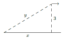
A plane is flying directly away from you at 500 mph at an altitude of 3 miles. How fast is the plane's distance from you increasing at the moment when the plane is flying over a point on the ground 4 miles from you?
To see what's going on, we first draw a schematic representation of the situation, as in figure 6.2.1.

Because the plane is in level flight directly away from you, the rate at which \(x\) changes is the speed of the plane, \(dx/dt=500\). The distance between you and the plane is \(y\); it is \(dy/dt\) that we wish to know. By the Pythagorean Theorem we know that \( x^2+9=y^2\). Taking the derivative:
\[ 2x \dot x = 2y\dot y. \nonumber \]
We are interested in the time at which \(x=4\); at this time we know that \(4^2+9=y^2\), so \(y=5\). Putting together all the information we get
\[2(4)(500)=2(5)\dot y. \nonumber \]
Thus, \( \dot y=400\) mph.
You are inflating a spherical balloon at the rate of 7 cm\({}^3\)/sec. How fast is its radius increasing when the radius is 4 cm?
Here the variables are the radius \(r\) and the volume \(V\). We know \(dV/dt\), and we want \(dr/dt\). The two variables are related by means of the equation \( V=4\pi r^3/3\). Taking the derivative of both sides gives \( dV/dt=4\pi r^2\dot r\). We now substitute the values we know at the instant in question: \( 7=4\pi
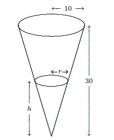
Water is poured into a conical container at the rate of 10 cm\({}^3\)/sec. The cone points directly down, and it has a height of 30 cm and a base radius of 10 cm; see figure 6.2.2. How fast is the water level rising when the water is 4 cm deep (at its deepest point)?
The water forms a conical shape within the big cone; its height and base radius and volume are all increasing as water is poured into the container. This means that we actually have three things varying with time: the water level \(h\) (the height of the cone of water), the radius \(r\) of the circular top surface of water (the base radius of the cone of water), and the volume of water \(V\). The volume of a cone is given by \( V=\pi r^2h/3\). We know \(dV/dt\), and we want \(dh/dt\). At first something seems to be wrong: we have a third variable \(r\) whose rate we don't know.

But the dimensions of the cone of water must have the same proportions as those of the container. That is, because of similar triangles, \(r/h=10/30\) so \(r=h/3\). Now we can eliminate \(r\) from the problem entirely: \( V=\pi(h/3)^2h/3=\pi h^3/27\). We take the derivative of both sides and plug in \(h=4\) and \(dV/dt=10\), obtaining \( 10=(3\pi\cdot 4^2/27)(dh/dt)\). Thus, \(dh/dt=90/(16\pi)\) cm/sec.
A swing consists of a board at the end of a 10 ft long rope. Think of the board as a point \(P\) at the end of the rope, and let \(Q\) be the point of attachment at the other end. Suppose that the swing is directly below \(Q\) at time \(t=0\), and is being pushed by someone who walks at 6 ft/sec from left to right. Find (a) how fast the swing is rising after 1 sec; (b) the angular speed of the rope in deg/sec after 1 sec.
We start out by asking: What is the geometric quantity whose rate of change we know, and what is the geometric quantity whose rate of change we're being asked about? Note that the person pushing the swing is moving horizontally at a rate we know. In other words, the horizontal coordinate of \(P\) is increasing at 6 ft/sec. In the \(xy\)-plane let us make the convenient choice of putting the origin at the location of \(P\) at time \(t=0\), i.e., a distance 10 directly below the point of attachment. Then the rate we know is \(dx/dt\), and in part (a) the rate we want is \(dy/dt\) (the rate at which \(P\) is rising). In part (b) the rate we want is \( \dot{\theta}=d\theta/dt\), where \(\theta\) stands for the angle in radians through which the swing has swung from the vertical. (Actually, since we want our answer in deg/sec, at the end we must convert \(d\theta/dt\) from rad/sec by multiplying by \(180/\pi\).)

(a) From the diagram we see that we have a right triangle whose legs are \(x\) and \(10-y\), and whose hypotenuse is 10. Hence \( x^2+(10-y)^2=100\). Taking the derivative of both sides we obtain: \(2x\dot{x}+2(10-y)(0-\dot{y})=0\). We now look at what we know after 1 second, namely \(x=6\) (because \(x\) started at 0 and has been increasing at the rate of 6 ft/sec for 1 sec), \(y=2\) (because we get \(10-y=8\) from the Pythagorean theorem applied to the triangle with hypotenuse 10 and leg 6), and \( \dot{x}=6\). Putting in these values gives us \(2\cdot 6\cdot 6-2\cdot 8\dot{y}=0\), from which we can easily solve for \( \dot{y}\): \( \dot{y}=4.5\) ft/sec.
(b) Here our two variables are \(x\) and \(\theta\), so we want to use the same right triangle as in part (a), but this time relate \(\theta\) to \(x\). Since the hypotenuse is constant (equal to 10), the best way to do this is to use the sine: \(\sin\theta=x/10\). Taking derivatives we obtain \( (\cos\theta)\dot{\theta}=0.1\dot{x}\). At the instant in question (\(t=1\) sec), when we have a right triangle with sides 6--8--10, \( \cos\theta=8/10\) and \( \dot{x}=6\). Thus \((8/10)\dot{\theta}=6/10\), i.e., \( \dot{\theta}=6/8=3/4\) rad/sec, or approximately \(43\) deg/sec.
We have seen that sometimes there are apparently more than two variables that change with time, but in reality there are just two, as the others can be expressed in terms of just two. But sometimes there really are several variables that change with time; as long as you know the rates of change of all but one of them you can find the rate of change of the remaining one. As in the case when there are just two variables, take the derivative of both sides of the equation relating all of the variables, and then substitute all of the known values and solve for the unknown rate.
A road running north to south crosses a road going east to west at the point \(P\). Car A is driving north along the first road, and car B is driving east along the second road. At a particular time car A is \(10\) kilometers to the north of \(P\) and traveling at 80 km/hr, while car B is 15 kilometers to the east of \(P\) and traveling at 100 km/hr. How fast is the distance between the two cars changing?

Let \(a(t)\) be the distance of car A north of \(P\) at time \(t\), and \(b(t)\) the distance of car B east of \(P\) at time \(t\), and let \(c(t)\) be the distance from car A to car B at time \(t\). By the Pythagorean Theorem, \( c(t)^2=a(t)^2+b(t)^2\). Taking derivatives we get \( 2c(t)c'(t)=2a(t)a'(t)+2b(t)b'(t)\), so
\[ \dot{c}={a\dot{a}+b\dot{b}\over c}={a\dot{a}+b\dot{b}\over \sqrt{a^2+b^2}}. \nonumber \]
Substituting known values we get:
\[ \dot{c}={10\cdot 80+15\cdot100\over \sqrt{10^2+15^2}}={460\over\sqrt{13}} \approx 127.6 \hbox{km/hr} \nonumber \]
at the time of interest.
Notice how this problem differs from example 6.2.2. In both cases we started with the Pythagorean Theorem and took derivatives on both sides. However, in example 6.2.2 one of the sides was a constant (the altitude of the plane), and so the derivative of the square of that side of the triangle was simply zero. In this example, on the other hand, all three sides of the right triangle are variables, even though we are interested in a specific value of each side of the triangle (namely, when the sides have lengths 10 and 15). Make sure that you understand at the start of the problem what are the variables and what are the constants.


