6.3: Newton's Method

Last updated
Save as PDF

Page ID: 448

$ \newcommand{\vecs}[1]{\overset { \scriptstyle \rightharpoonup} {\mathbf{#1}} } $

$ \newcommand{\vecd}[1]{\overset{-\!-\!\rightharpoonup}{\vphantom{a}\smash {#1}}} $

$ \newcommand{\id}{\mathrm{id}}$ $ \newcommand{\Span}{\mathrm{span}}$

( \newcommand{\kernel}{\mathrm{null}\,}\) $ \newcommand{\range}{\mathrm{range}\,}$

$ \newcommand{\RealPart}{\mathrm{Re}}$ $ \newcommand{\ImaginaryPart}{\mathrm{Im}}$

$ \newcommand{\Argument}{\mathrm{Arg}}$ $ \newcommand{\norm}[1]{\| #1 \|}$

$ \newcommand{\inner}[2]{\langle #1, #2 \rangle}$

$ \newcommand{\Span}{\mathrm{span}}$

$ \newcommand{\id}{\mathrm{id}}$

$ \newcommand{\Span}{\mathrm{span}}$

$ \newcommand{\kernel}{\mathrm{null}\,}$

$ \newcommand{\range}{\mathrm{range}\,}$

$ \newcommand{\RealPart}{\mathrm{Re}}$

$ \newcommand{\ImaginaryPart}{\mathrm{Im}}$

$ \newcommand{\Argument}{\mathrm{Arg}}$

$ \newcommand{\norm}[1]{\| #1 \|}$

$ \newcommand{\inner}[2]{\langle #1, #2 \rangle}$

$ \newcommand{\Span}{\mathrm{span}}$ $ \newcommand{\AA}{\unicode[.8,0]{x212B}}$

$ \newcommand{\vectorA}[1]{\vec{#1}} % arrow$

$ \newcommand{\vectorAt}[1]{\vec{\text{#1}}} % arrow$

$ \newcommand{\vectorB}[1]{\overset { \scriptstyle \rightharpoonup} {\mathbf{#1}} } $

$ \newcommand{\vectorC}[1]{\textbf{#1}} $

$ \newcommand{\vectorD}[1]{\overrightarrow{#1}} $

$ \newcommand{\vectorDt}[1]{\overrightarrow{\text{#1}}} $

$ \newcommand{\vectE}[1]{\overset{-\!-\!\rightharpoonup}{\vphantom{a}\smash{\mathbf {#1}}}} $

$ \newcommand{\vecs}[1]{\overset { \scriptstyle \rightharpoonup} {\mathbf{#1}} } $

$ \newcommand{\vecd}[1]{\overset{-\!-\!\rightharpoonup}{\vphantom{a}\smash {#1}}} $

$\newcommand{\avec}{\mathbf a}$ $\newcommand{\bvec}{\mathbf b}$ $\newcommand{\cvec}{\mathbf c}$ $\newcommand{\dvec}{\mathbf d}$ $\newcommand{\dtil}{\widetilde{\mathbf d}}$ $\newcommand{\evec}{\mathbf e}$ $\newcommand{\fvec}{\mathbf f}$ $\newcommand{\nvec}{\mathbf n}$ $\newcommand{\pvec}{\mathbf p}$ $\newcommand{\qvec}{\mathbf q}$ $\newcommand{\svec}{\mathbf s}$ $\newcommand{\tvec}{\mathbf t}$ $\newcommand{\uvec}{\mathbf u}$ $\newcommand{\vvec}{\mathbf v}$ $\newcommand{\wvec}{\mathbf w}$ $\newcommand{\xvec}{\mathbf x}$ $\newcommand{\yvec}{\mathbf y}$ $\newcommand{\zvec}{\mathbf z}$ $\newcommand{\rvec}{\mathbf r}$ $\newcommand{\mvec}{\mathbf m}$ $\newcommand{\zerovec}{\mathbf 0}$ $\newcommand{\onevec}{\mathbf 1}$ $\newcommand{\real}{\mathbb R}$ $\newcommand{\twovec}[2]{\left[\begin{array}{r}#1 \\ #2 \end{array}\right]}$ $\newcommand{\ctwovec}[2]{\left[\begin{array}{c}#1 \\ #2 \end{array}\right]}$ $\newcommand{\threevec}[3]{\left[\begin{array}{r}#1 \\ #2 \\ #3 \end{array}\right]}$ $\newcommand{\cthreevec}[3]{\left[\begin{array}{c}#1 \\ #2 \\ #3 \end{array}\right]}$ $\newcommand{\fourvec}[4]{\left[\begin{array}{r}#1 \\ #2 \\ #3 \\ #4 \end{array}\right]}$ $\newcommand{\cfourvec}[4]{\left[\begin{array}{c}#1 \\ #2 \\ #3 \\ #4 \end{array}\right]}$ $\newcommand{\fivevec}[5]{\left[\begin{array}{r}#1 \\ #2 \\ #3 \\ #4 \\ #5 \\ \end{array}\right]}$ $\newcommand{\cfivevec}[5]{\left[\begin{array}{c}#1 \\ #2 \\ #3 \\ #4 \\ #5 \\ \end{array}\right]}$ $\newcommand{\mattwo}[4]{\left[\begin{array}{rr}#1 \amp #2 \\ #3 \amp #4 \\ \end{array}\right]}$ $\newcommand{\laspan}[1]{\text{Span}\{#1\}}$ $\newcommand{\bcal}{\cal B}$ $\newcommand{\ccal}{\cal C}$ $\newcommand{\scal}{\cal S}$ $\newcommand{\wcal}{\cal W}$ $\newcommand{\ecal}{\cal E}$ $\newcommand{\coords}[2]{\left\{#1\right\}_{#2}}$ $\newcommand{\gray}[1]{\color{gray}{#1}}$ $\newcommand{\lgray}[1]{\color{lightgray}{#1}}$ $\newcommand{\rank}{\operatorname{rank}}$ $\newcommand{\row}{\text{Row}}$ $\newcommand{\col}{\text{Col}}$ $\renewcommand{\row}{\text{Row}}$ $\newcommand{\nul}{\text{Nul}}$ $\newcommand{\var}{\text{Var}}$ $\newcommand{\corr}{\text{corr}}$ $\newcommand{\len}[1]{\left|#1\right|}$ $\newcommand{\bbar}{\overline{\bvec}}$ $\newcommand{\bhat}{\widehat{\bvec}}$ $\newcommand{\bperp}{\bvec^\perp}$ $\newcommand{\xhat}{\widehat{\xvec}}$ $\newcommand{\vhat}{\widehat{\vvec}}$ $\newcommand{\uhat}{\widehat{\uvec}}$ $\newcommand{\what}{\widehat{\wvec}}$ $\newcommand{\Sighat}{\widehat{\Sigma}}$ $\newcommand{\lt}{<}$ $\newcommand{\gt}{>}$ $\newcommand{\amp}{&}$ $\definecolor{fillinmathshade}{gray}{0.9}$

Suppose you have a function $f(x)$, and you want to find as accurately as possible where it crosses the $x$-axis; in other words, you want to solve $f(x)=0$. Suppose you know of no way to find an exact solution by any algebraic procedure, but you are able to use an approximation, provided it can be made quite close to the true value. Newton's method is a way to find a solution to the equation to as many decimal places as you want. It is what is called an "iterative procedure,'' meaning that it can be repeated again and again to get an answer of greater and greater accuracy. Iterative procedures like Newton's method are well suited to programming for a computer. Newton's method uses the fact that the tangent line to a curve is a good approximation to the curve near the point of tangency.

Example $\PageIndex{1}$

Approximate $ \sqrt{3}$.

Solution

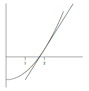
Since $ \sqrt{3}$ is a solution to $ x^2=3$ or $x^2-3=0$, we use $ f(x)=x^2-3$. We start by guessing something reasonably close to the true value; this is usually easy to do; let's use $ \sqrt3\approx2$. Now use the tangent line to the curve when $x=2$ as an approximation to the curve, as shown in Figure $\PageIndex{1}$.

$alt$

Figure $\PageIndex{1}$: Netwon's Method

Since $f'(x)=2x$, the slope of this tangent line is 4 and its equation is $y=4x-7$. The tangent line is quite close to $f(x)$, so it crosses the $x$-axis near the point at which $f(x)$ crosses, that is, near $ \sqrt3$. It is easy to find where the tangent line crosses the $x$-axis: solve $0=4x-7$ to get $x=7/4=1.75$. This is certainly a better approximation than 2, but let us say not close enough. We can improve it by doing the same thing again: find the tangent line at $x=1.75$, find where this new tangent line crosses the $x$-axis, and use that value as a better approximation. We can continue this indefinitely, though it gets a bit tedious. Lets see if we can shortcut the process. Suppose the best approximation to the intercept we have so far is $ x_i$. To find a better approximation we will always do the same thing: find the slope of the tangent line at $ x_i$, find the equation of the tangent line, find the $x$-intercept. The slope is $ 2x_i$. The tangent line is

\[ y=(2x_i)(x-x_i)+(x_i^2-3),\]

using the point-slope formula for a line. Finally, the intercept is found by solving

\[ 0 =(2x_i)(x-x_i)+(x_i^2-3). \label{EX1b}\]

With a little algebra, Equation \ref{EX1b} turns into

\[ x= \dfrac{x_i^2+3}{2x_i}\]

this is the next approximation, which we naturally call $x_{i+1}$. Instead of doing the whole tangent line computation every time we can simply use this formula to get as many approximations as we want.

Starting with $ x_0=2$, we get

\[ x_1=\dfrac{x_0^2+3}{2x_0}=\dfrac{2^2+3}{4}=\dfrac{7}{4}\]

(the same approximation we got above, of course),

\[ x_2=\dfrac{x_1^2+3}{2x_1}= \dfrac{(7/4)^2+3}{(7/2)}=\dfrac{97}{56}\approx 1.73214,\]

and

\[ x_3\approx 1.73205,\]

and so on. This is still a bit tedious by hand, but with a calculator or, even better, a good computer program, it is quite easy to get many, many approximations. We might guess already that $1.73205$ is accurate to two decimal places, and in fact it turns out that it is accurate to 5 places.

Let's think about this process in more general terms. We want to approximate a solution to $f(x)=0$. We start with a rough guess, which we call $ x_0$. We use the tangent line to $f(x)$ to get a new approximation that we hope will be closer to the true value. What is the equation of the tangent line when $ x=x_0$? The slope is $ f'(x_0)$ and the line goes through $(x_0,f(x_0))$, so the equation of the line is

\[ y=f'(x_0)(x-x_0)+f(x_0).\]

Now we find where this crosses the $x$-axis by substituting $y=0$ and solving for $x$: $$x={x_0f'(x_0)-f(x_0)\over f'(x_0)} = x_0 - {f(x_0)\over f'(x_0)}.$$ We will typically want to compute more than one of these improved approximations, so we number them consecutively; from $ x_0$ we have computed $ x_1$:

\[x_1={x_0f'(x_0)-f(x_0)\over f'(x_0)} = x_0 - {f(x_0)\over f'(x_0)},\]

and in general from $ x_i$ we compute $ x_{i+1}$:

\[x_{i+1}={x_if'(x_i)-f(x_i)\over f'(x_i)} = x_i - {f(x_i)\over f'(x_i)}.\]

$\PageIndex{2}$

Returning to the Example $\PageIndex{1}$, $ f(x)=x^2-3$, $f'(x)=2x$, and the formula becomes

\[ x_{i+1}=x_i - \dfrac{x_i^2-3}{2x_i}=\dfrac{x_i^2+3}{2x_i}\]

as before.

In practice, which is to say, if you need to approximate a value in the course of designing a bridge or a building or an airframe, you will need to have some confidence that the approximation you settle on is accurate enough. As a rule of thumb, once a certain number of decimal places stop changing from one approximation to the next it is likely that those decimal places are correct. Still, this may not be enough assurance, in which case we can test the result for accuracy.

$\PageIndex{3}$

Find the $x$ coordinate of the intersection of the curves $y=2x$ and $y=\tan x$, accurate to three decimal places.

Solution

To put this in the context of Newton's method, we note that we want to know where $2x=\tan x$ or $f(x)=\tan x-2x=0$. We compute $ f'(x)=\sec^2 x - 2$ and set up the formula:

\[x_{i+1} = x_i-{\tan x_i -2x_i\over \sec^2 x_i - 2}.\]

$alt$

Figure $\PageIndex{2}$. $y=\tan x$ and $y=2x$ on the left, $y=\tan x -2x$

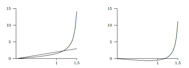
From the graph in Figure $\PageIndex{2}$ we guess $ x_0=1$ as a starting point, then using the formula we compute

$ x_1=1.310478030$,
$ x_2=1.223929096$,
$ x_3=1.176050900$,
$ x_4=1.165926508$,
$ x_5=1.165561636$.

So we guess that the first three places are correct, but that is not the same as saying $1.165$ is correct to three decimal places---$1.166$ might be the correct, rounded approximation. How can we tell? We can substitute 1.165, 1.1655 and 1.166 into $\tan x - 2x$; this gives -0.002483652, -0.000271247, 0.001948654. Since the first two are negative and the third is positive, $\tan x - 2x$ crosses the $x$ axis between 1.1655 and 1.166, so the correct value to three places is 1.166.

Contributors

- Integrated by Justin Marshall.

Search

Text Color

Text Size

Margin Size

Font Type