
10.1: Polar Coordinates
- Page ID
- 515

Coordinate systems are tools that let us use algebraic methods to understand geometry. While the rectangular (also called Cartesian) coordinates that we have been using are the most common, some problems are easier to analyze in alternate coordinate systems.
A coordinate system is a scheme that allows us to identify any point in the plane or in three-dimensional space by a set of numbers. In rectangular coordinates these numbers are interpreted, roughly speaking, as the lengths of the sides of a rectangle. In polar coordinates a point in the plane is identified by a pair of numbers \((r,\theta)\). The number \(\theta\) measures the angle between the positive \(x\)-axis and a ray that goes through the point, as shown in figure 10.1.1; the number \(r\) measures the distance from the origin to the point. Figure 10.1.1 shows the point with rectangular coordinates \( (1,\sqrt3)\) and polar coordinates \((2,\pi/3)\), 2 units from the origin and \(\pi/3\) radians from the positive \(x\)-axis.
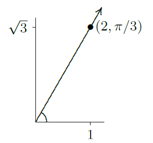
Figure 10.1.1. Polar coordinates of the point \((1,\sqrt3)\).
Just as we describe curves in the plane using equations involving \(x\) and \(y\), so can we describe curves using equations involving \(r\) and \(\theta\). Most common are equations of the form \(r=f(\theta)\).
All points with \(r=2\) are at distance 2 from the origin, so \(r=2\) describes the circle of radius 2 with center at the origin. Just as we describe curves in the plane using equations involving \(x\) and \(y\), so can we describe curves using equations involving \(r\) and \(\theta\). Most common are equations of the form \(r=f(\theta)\).
also has coordinates \((2,5\pi/4)\) and \((2,-3\pi/4)\).
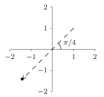
Figure 10.1.3. The point \((-2,\pi/4)=(2,5\pi/4)=(2,-3\pi/4)\) in polar coordinates.
The relationship between rectangular and polar coordinates is quite easy to understand. The point with polar coordinates \((r,\theta)\) has rectangular coordinates \(x=r\cos\theta\) and \(y=r\sin\theta\); this follows immediately from the definition of the sine and cosine functions. Using figure 10.1.3 as an example, the point shown has rectangular coordinates \(x=(-2)\cos(\pi/4)=-\sqrt2\approx 1.4142\) and \( y=(-2)\sin(\pi/4)=-\sqrt2\). This makes it very easy to convert equations from rectangular to polar coordinates.
We merely substitute: \(r\sin\theta=3r\cos\theta+2\), or \(r= {2\over \sin\theta-3\cos\theta}\).
Again substituting: \((r\cos\theta-1/2)^2+r^2\sin^2\theta=1/4\). A bit of algebra turns this into \(r=\cos(t)\). You should try plotting a few \((r,\theta)\) values to convince yourself that this makes sense.
. When \(\theta < 0\), \(r\) is also negative, and so the full graph is the right hand picture in the figure.
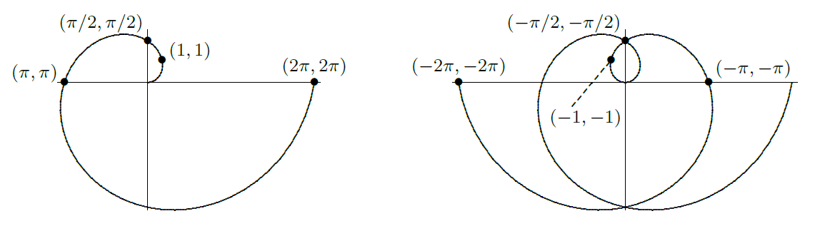
Figure 10.1.4. The spiral of Archimedes and the full graph of \(r=\theta\).
Converting polar equations to rectangular equations can be somewhat trickier, and graphing polar equations directly is also not always easy.
. Now, this suggests that the curve could possibly be a circle, and if it is, it would have to be the circle \(x^2+(y-1)^2=1\). Having made this guess, we can easily check it. First we substitute for \(x\) and \(y\) to get \((r\cos\theta)^2+(r\sin\theta-1)^2=1\); expanding and simplifying does indeed turn this into \(r=2\sin\theta\).
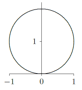
Figure 10.1.5. Graph of \(r=2\sin\theta\).
Contributors and Attributions
Integrated by Justin Marshall.