14.2: Limits and Continuity

To develop calculus for functions of one variable, we needed to make sense of the concept of a limit, which we needed to understand continuous functions and to define the derivative. Limits involving functions of two variables can be considerably more difficult to deal with; fortunately, most of the functions we encounter are fairly easy to understand.

The potential difficulty is largely due to the fact that there are many ways to "approach'' a point in the \(x\)-\(y\) plane. If we want to say that \( \lim_{(x,y)\to(a,b)}f(x,y)=L\), we need to capture the idea that as \((x,y)\) gets close to \((a,b)\) then \(f(x,y)\) gets close to \(L\). For functions of one variable, \(f(x)\), there are only two ways that \(x\) can approach \(a\): from the left or right. But there are an infinite number of ways to approach \((a,b)\): along any one of an infinite number of lines, or an infinite number of parabolas, or an infinite number of sine curves, and so on. We might hope that it's really not so bad---suppose, for example, that along every possible line through \((a,b)\) the value of \(f(x,y)\) gets close to \(L\); surely this means that "\(f(x,y)\) approaches \(L\) as \((x,y)\) approaches \((a,b)\)''. Sadly, no.

Figure 14.2.1. \( f(x,y)={xy^2\over x^2+y^4}\)

Example 14.2.1

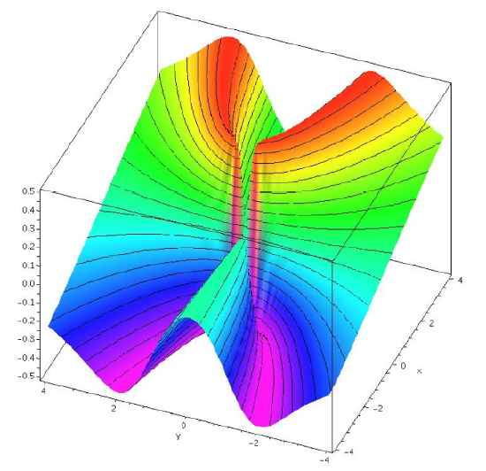
Consider \(f(x,y)=xy^2/(x^2+y^4)\). When \(x=0\) or \(y=0\), \(f(x,y)\) is 0, so the limit of \(f(x,y)\) approaching the origin along either the \(x\) or \(y\) axis is 0. Moreover, along the line \(y=mx\), \(f(x,y)=m^2x^3/(x^2+m^4x^4)\). As \(x\) approaches 0 this expression approaches 0 as well. So along every line through the origin \(f(x,y)\) approaches 0. Now suppose we approach the origin along \(x=y^2\). Then \[f(x,y)={y^2y^2\over y^4+y^4}={y^4\over2y^4}={1\over2},\] so the limit is \(1/2\). Looking at figure 14.2.1, it is apparent that there is a ridge above \(x=y^2\). Approaching the origin along a straight line, we go over the ridge and then drop down toward 0, but approaching along the ridge the height is a constant \(1/2\).

Fortunately, we can define the concept of limit without needing to specify how a particular point is approached---indeed, in definition 2.3.2, we didn't need the concept of "approach.'' Roughly, that definition says that when \(x\) is close to \(a\) then \(f(x)\) is close to \(L\); there is no mention of "how'' we get close to \(a\). We can adapt that definition to two variables quite easily:'

Definition 14.2.2: Limits

(Limit) Suppose \(f(x,y)\) is a function. We say that \[\lim_{(x,y)\to (a,b)}f(x,y)=L\] if for every \(\epsilon>0\) there is a \(\delta > 0\) so that whenever \(0 < \sqrt{(x-a)^2+(y-b)^2} < \delta\), \(|f(x,y)-L| < \epsilon\).

This says that we can make \(|f(x,y)-L| < \epsilon\), no matter how small \(\epsilon\) is, by making the distance from \((x,y)\) to \((a,b)\) "small enough''.

Example 14.2.3

We show that \( \lim_{(x,y)\to(0,0)}{3x^2y\over x^2+y^2}=0\). Suppose \(\epsilon>0\). Then \[\left|{3x^2y\over x^2+y^2}\right|={x^2\over x^2+y^2}3|y|.\] Note that \(x^2/(x^2+y^2)\le1\) and \(|y|=\sqrt{y^2}\le\sqrt{x^2+y^2} < \delta\). So \[{x^2\over x^2+y^2}3|y| < 1\cdot 3\cdot \delta.\] We want to force this to be less than \(\epsilon\) by picking \(\delta\) "small enough.'' If we choose \(\delta=\epsilon/3\) then \[\left|{3x^2y\over x^2+y^2}\right| < 1\cdot 3\cdot{\epsilon\over3}= \epsilon.\]

Recall that a function \(f(x)\) is continuous at \(x=a\) if \( \lim_{x\to a}f(x)=f(a)\); roughly this says that there is no "hole'' or "jump'' at \(x=a\). We can say exactly the same thing about a function of two variables: \(f(x,y)\) is continuous at \((a,b)\) if \( \lim_{(x,y)\to (a,b)}f(x,y)=f(a,b)\).

Example

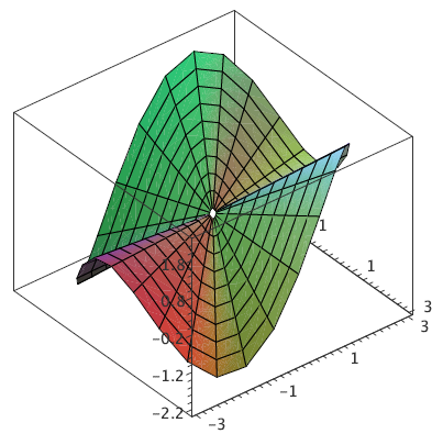
Example 14.2.4 The function \(f(x,y)=3x^2y/(x^2+y^2)\) is not continuous at \((0,0)\), because \(f(0,0)\) is not defined. However, we know that \( \lim_{(x,y)\to(0,0)}f(x,y)=0\), so we can easily "fix'' the problem, by extending the definition of \(f\) so that \(f(0,0)=0\). This surface is shown in figure 14.2.2.

Figure 14.2.2. \( f(x,y)={3x^2y\over x^2+y^2}\)

Note that in contrast to this example we cannot fix example 14.2.1 at \((0,0)\) because the limit does not exist. No matter what value we try to assign to \(f\) at \((0,0)\) the surface will have a "jump'' there.

Fortunately, the functions we will examine will typically be continuous almost everywhere. Usually this follows easily from the fact that closely related functions of one variable are continuous. As with single variable functions, two classes of common functions are particularly useful and easy to describe. A polynomial in two variables is a sum of terms of the form \(ax^my^n\), where \(a\) is a real number and \(m\) and \(n\) are non-negative integers. A rational function is a quotient of polynomials.

Theorem 14.2.5

Polynomials are continuous everywhere. Rational functions are continuous everywhere they are defined.

Contributors

• David Guichard (Whitman College)

• Integrated by Justin Marshall.