17.5: Second Order Homogeneous Equations

A second order differential equation is one containing the second derivative. These are in general quite complicated, but one fairly simple type is useful: the second order linear equation with constant coefficients.

Example $\PageIndex{1}$:

Consider the intial value problem $\ddot y-\dot y-2y=0$, $y(0)=5$, $\dot y(0)=0$. We make an inspired guess: might there be a solution of the form $e^{rt}$? This seems at least plausible, since in this case $\ddot y$, $\dot y$, and $y$ all involve $e^{rt}$.

If such a function is a solution then

$$\eqalign{ r^2 e^{rt}-r e^{rt}-2e^{rt}&=0\cr e^{rt}(r^2-r-2)&=0\cr (r^2-r-2)&=0\cr (r-2)(r+1)&=0,\cr}$$

so $r$ is $2$ or $-1$. Not only are $f=e^{2t}$ and $g=e^{-t}$ solutions, but notice that $y=Af+Bg$ is also, for any constants $A$ and $B$:

$$\eqalign{ (Af+Bg)''-(Af+Bg)'-2(Af+Bg)&=Af''+Bg''-Af'-Bg'-2Af-2Bg\cr &=A(f''-f'-2f)+B(g''-g'-2g)\cr &=A(0)+B(0)=0.\cr}$$

Can we find $A$ and $B$ so that this is a solution to the initial value problem? Let's substitute:

$$5=y(0)=Af(0)+Bg(0)=Ae^0+Be^0=A+B$$

and

$$0=\dot y(0)=Af'(0)+Bg'(0)=A2e^{0}+B(-1)e^0=2A-B.$$

So we need to find $A$ and $B$ that make both $5=A+B$ and $0=2A-B$ true. This is a simple set of simultaneous equations: solve $B=2A$, substitute to get $5=A+2A=3A$. Then $A=5/3$ and $B=10/3$, and the desired solution is $(5/3)e^{2t}+(10/3)e^{-t}$. You now see why the initial condition in this case included both $y(0)$ and $\dot y(0)$: we needed two equations in the two unknowns $A$ and $B$

You should of course wonder whether there might be other solutions; the answer is no. We will not prove this, but here is the theorem that tells us what we need to know:

Theorem 17.5.2

Given the differential equation $a\ddot y+b\dot y+cy=0$, $a\not=0$, consider the quadratic polynomial $ax^2+bx+c$, called the characteristic polynomial. Using the quadratic formula, this polynomial always has one or two roots, call them $r$ and $s$. The general solution of the differential equation is

a. $y=Ae^{rt}+Be^{st}$, if the roots $r$ and $s$ are real numbers and $r\not=s$.

b. $y=Ae^{rt}+Bte^{rt}$, if $r=s$ is real.

c. $y=A\cos(\beta t)e^{\alpha t}+B\sin(\beta t)e^{\alpha t}$, if the roots $r$ and $s$ are complex numbers $\alpha+\beta i$ and $\alpha-\beta i$

Example $\PageIndex{3}$:

Suppose a mass $m$ is hung on a spring with spring constant $k$. If the spring is compressed or stretched and then released, the mass will oscillate up and down. Because of friction, the oscillation will be damped: eventually the motion will cease. The damping will depend on the amount of friction; for example, if the system is suspended in oil the motion will cease sooner than if the system is in air. Using some simple physics, it is not hard to see that the position of the mass is described by this differential equation: $m\ddot y+b\dot y+ky=0$. Using $m=1$, $b=4$, and $k=5$ we find the motion of the mass. The characteristic polynomial is $x^2+4x+5$ with roots $(-4\pm\sqrt{16-20})/2=-2\pm i$. Thus the general solution is $y=A\cos(t)e^{-2t}+B\sin(t)e^{-2t}$. Suppose we know that $y(0)=1$ and $\dot y(0)=2$. Then as before we form two simultaneous equations: from $y(0)=1$ we get $1=A\cos(0)e^0+B\sin(0)e^0=A$. For the second we compute

$$\ddot y=-2Ae^{-2t}\cos(t)+Ae^{-2t}(-\sin(t))-2Be^{-2t}\sin(t)+Be^{-2t}\cos(t),$$

and then

$$2=-2Ae^0\cos(0)-Ae^0\sin(0)-2Be^0\sin(0)+Be^0\cos(0)=-2A+B.$$

So we get $A=1$, $B=4$, and $y=\cos(t)e^{-2t}+4\sin(t)e^{-2t}$. Here is a useful trick that makes this easier to understand: We have $y=(\cos t+4\sin t)e^{-2t}$. The expression $\cos t+4 \sin t$ is a bit reminiscent of the trigonometric formula $\cos(\alpha-\beta)=\cos(\alpha)\cos(\beta)+\sin(\alpha)\sin(\beta)$ with $\alpha=t$. Let's rewrite it a bit as

$$\sqrt{17}\left({1\over\sqrt{17}}\cos t + {4\over\sqrt{17}}\sin t\right).$$

Note that $(1/\sqrt{17})^2+(4/\sqrt{17})^2=1$, which means that there is an angle $\beta$ with $\cos\beta=1/\sqrt{17}$ and $\sin\beta=4/\sqrt{17}$ (of course, $\beta$ may not be a "nice" angle). Then

$$\cos t+4\sin t = \sqrt{17}\left(\cos t\cos \beta+\sin\beta\sin t\right) =\sqrt{17}\cos(t-\beta).$$

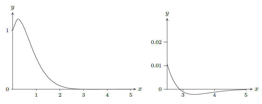
Thus, the solution may also be written $y=\sqrt{17}e^{-2t}\cos(t-\beta)$. This is a cosine curve that has been shifted $\beta$ to the right; the $\sqrt{17}e^{-2t}$ has the effect of diminishing the amplitude of the cosine as $t$ increases; see figure 17.5.1. The oscillation is damped very quickly, so in the first graph it is not clear that this is an oscillation. The second graph shows a restricted range for $t$.

Other physical systems that oscillate can also be described by such differential equations. Some electric circuits, for example, generate oscillating current.

Figure 17.5.1. Graph of a Dampened Oscillator

Example $\PageIndex{1}$:

Find the solution to the intial value problem $\ddot y-4\dot y+4y=0$, $y(0)=-3$, $\dot y(0)=1$.

Solution

The characteristic polynomial is $x^2-4x+4=(x-2)^2$, so there is one root, $r=2$, and the general solution is $Ae^{2t}+Bte^{2t}$. Substituting $t=0$ we get $-3=A+0=A$. The first derivative is $2Ae^{2t}+2Bte^{2t}+Be^{2t}$; substituting $t=0$ gives $1=2A+0+B=2A+B=2(-3)+B=-6+B$, so $B=7$. The solution is $-3e^{2t}+7te^{2t}$.

Contributors

• David Guichard (Whitman College)

• Integrated by Justin Marshall.