14.3: Partial Derivatives

Learning Objectives

• Calculate the partial derivatives of a function of two variables.
• Calculate the partial derivatives of a function of more than two variables.
• Determine the higher-order derivatives of a function of two variables.
• Explain the meaning of a partial differential equation and give an example.

Now that we have examined limits and continuity of functions of two variables, we can proceed to study derivatives. Finding derivatives of functions of two variables is the key concept in this chapter, with as many applications in mathematics, science, and engineering as differentiation of single-variable functions. However, we have already seen that limits and continuity of multivariable functions have new issues and require new terminology and ideas to deal with them. This carries over into differentiation as well.

Derivatives of a Function of Two Variables

When studying derivatives of functions of one variable, we found that one interpretation of the derivative is an instantaneous rate of change of $y$ as a function of $x.$ Leibniz notation for the derivative is $dy/dx,$ which implies that $y$ is the dependent variable and $x$ is the independent variable. For a function $z=f(x,y)$ of two variables, $x$ and $y$ are the independent variables and $z$ is the dependent variable. This raises two questions right away: How do we adapt Leibniz notation for functions of two variables? Also, what is an interpretation of the derivative? The answer lies in partial derivatives.

Definition: Partial Derivatives

Let $f(x,y)$ be a function of two variables. Then the partial derivative of $f$ with respect to $x$, written as $∂f/∂x,$, or $f_x,$ is defined as

$$\dfrac{∂f}{∂x}=f_x(x,y)=\lim_{h→0}\dfrac{f(x+h,y)−f(x,y)}{h} \label{pd1}$$

The partial derivative of $f$ with respect to $y$, written as $∂f/∂y$, or $f_y,$ is defined as

$$\dfrac{∂f}{∂y}=f_y(x,y)=\lim_{k→0}\dfrac{f(x,y+k)−f(x,y)}{k}. \label{pd2}$$

This definition shows two differences already. First, the notation changes, in the sense that we still use a version of Leibniz notation, but the $d$ in the original notation is replaced with the symbol $∂$. (This rounded $“d”$ is usually called “partial,” so $∂f/∂x$ is spoken as the “partial of $f$ with respect to $x$.”) This is the first hint that we are dealing with partial derivatives. Second, we now have two different derivatives we can take, since there are two different independent variables. Depending on which variable we choose, we can come up with different partial derivatives altogether, and often do.

Example $\PageIndex{1}$: Calculating Partial Derivatives from the Definition

Use the definition of the partial derivative as a limit to calculate $∂f/∂x$ and $∂f/∂y$ for the function

$$f(x,y)=x^2−3xy+2y^2−4x+5y−12. \nonumber$$

Solution

First, calculate $f(x+h,y).$

$$\begin{align*} f(x+h,y) &=(x+h)^2−3(x+h)y+2y^2−4(x+h)+5y−12 \\ &=x^2+2xh+h^2−3xy−3hy+2y^2−4x−4h+5y−12. \end{align*} \nonumber$$

Next, substitute this into Equation $\ref{pd1}$ and simplify:

$$\begin{align*} \dfrac{∂f}{∂x} &=\lim_{h→0}\dfrac{f(x+h,y)−f(x,y)}{h} \\ &=\lim_{h→0}\dfrac{(x^2+2xh+h^2−3xy−3hy+2y^2−4x−4h+5y−12)−(x^2−3xy+2y^2−4x+5y−12)}{h} \\ &=\lim_{h→0}\dfrac{x^2+2xh+h^2−3xy−3hy+2y^2−4x−4h+5y−12−x^2+3xy−2y^2+4x−5y+12}{h} \\ &=\lim_{h→0}\dfrac{2xh+h^2−3hy−4h}{h}\\ &=\lim_{h→0}\dfrac{h(2x+h−3y−4)}{h} \\ &=\lim_{h→0}(2x+h−3y−4) \\ &=2x−3y−4. \end{align*}$$

To calculate $\dfrac{∂f}{∂y}$, first calculate $f(x,y+h):$

$$\begin{align*} f(x,y+h) &=x^2−3x(y+h)+2(y+h)^2−4x+5(y+h)−12 \\ &=x^2−3xy−3xh+2y^2+4yh+2h^2−4x+5y+5h−12. \end{align*}$$

Next, substitute this into Equation $\ref{pd2}$ and simplify:

$$\begin{align*} \dfrac{∂f}{∂y} &=\lim_{h→0}\dfrac{f(x,y+h)−f(x,y)}{h} \\ &=\lim_{h→0}\dfrac{(x^2−3xy−3xh+2y^2+4yh+2h^2−4x+5y+5h−12)−(x^2−3xy+2y^2−4x+5y−12)}{h} \\ &=\lim_{h→0}\dfrac{x^2−3xy−3xh+2y^2+4yh+2h^2−4x+5y+5h−12−x^2+3xy−2y^2+4x−5y+12}{h} \\ &=\lim_{h→0}\dfrac{−3xh+4yh+2h^2+5h}{h} \\ &=\lim_{h→0}\dfrac{h(−3x+4y+2h+5)}{h} \\ &=\lim_{h→0}(−3x+4y+2h+5) \\ &=−3x+4y+5 \end{align*}$$

Exercise $\PageIndex{1}$

Use the definition of the partial derivative as a limit to calculate $∂f/∂x$ and $∂f/∂y$ for the function

$$f(x,y)=4x^2+2xy−y^2+3x−2y+5.\nonumber$$

Hint

Use Equations $\ref{pd1}$ and $\ref{pd2}$ from the definition of partial derivatives.

Answer

$\dfrac{∂f}{∂x}=8x+2y+3$

$\dfrac{∂f}{∂y}=2x−2y−2$

The idea to keep in mind when calculating partial derivatives is to treat all independent variables, other than the variable with respect to which we are differentiating, as constants. Then proceed to differentiate as with a function of a single variable. To see why this is true, first fix $y$ and define $g(x)=f(x,y)$ as a function of $x$. Then

$$\begin{align*} g′(x) &=\lim_{h→0}\dfrac{g(x+h)−g(x)}{h} \\[6pt] &=\lim_{h→0}\dfrac{f(x+h,y)−f(x,y)}{h} \\[6pt] &=\dfrac{∂f}{∂x}. \end{align*}$$

The same is true for calculating the partial derivative of $f$ with respect to $y$. This time, fix $x$ and define $h(y)=f(x,y)$ as a function of $y$. Then

$$\begin{align*} h′(x) &=\lim_{k→0}\dfrac{h(x+k)−h(x)}{k} \\[6pt] &=\lim_{k→0}\dfrac{f(x,y+k)−f(x,y)}{k} \\[6pt] &=\dfrac{∂f}{∂y}. \end{align*}$$

All differentiation rules apply.

Example $\PageIndex{2}$: Calculating Partial Derivatives

Calculate $∂f/∂x$ and $∂f/∂y$ for the following functions by holding the opposite variable constant then differentiating:

1. $f(x,y)=x^2−3xy+2y^2−4x+5y−12$
2. $g(x,y)=\sin(x^2y−2x+4)$

Solution:

a. To calculate $∂f/∂x$, treat the variable $y$ as a constant. Then differentiate $f(x,y)$ with respect to $x$ using the sum, difference, and power rules:

$$\begin{align*}\dfrac{∂f}{∂x} &=\dfrac{∂}{∂x}\left[x^2−3xy+2y^2−4x+5y−12\right] \\[6pt] &=\dfrac{∂}{∂x}[x^2]−\dfrac{∂}{∂x}[3xy]+\dfrac{∂}{∂x}[2y^2]−\dfrac{∂}{∂x}[4x]+\dfrac{∂}{∂x}[5y]−\dfrac{∂}{∂x}[12] \\[6pt] &=2x−3y+0−4+0−0 \\ &=2x−3y−4. \end{align*}$$

The derivatives of the third, fifth, and sixth terms are all zero because they do not contain the variable $x$, so they are treated as constant terms. The derivative of the second term is equal to the coefficient of $x$, which is $−3y$. Calculating $∂f/∂y$:

$$\begin{align*} \dfrac{∂f}{∂y} &=\dfrac{∂}{∂y}\left[x^2−3xy+2y^2−4x+5y−12\right] \\[6pt] &=\dfrac{∂}{∂y}[x^2]−\dfrac{∂}{∂y}[3xy]+\dfrac{∂}{∂y}[2y^2]−\dfrac{∂}{∂y}[4x]+\dfrac{∂}{∂y}[5y]−\dfrac{∂}{∂y}[12] \\[6pt] &=0−3x+4y−0+5−0 \\ &=−3x+4y+5. \end{align*} \nonumber$$

These are the same answers obtained in Example $\PageIndex{1}$.

b. To calculate $∂g/∂x,$ treat the variable y as a constant. Then differentiate $g(x,y)$ with respect to $x$ using the chain rule and power rule:

$$\begin{align*}\dfrac{∂g}{∂x} &=\dfrac{∂}{∂x}\left[\sin(x^2y−2x+4)\right] \\[6pt] &=\cos(x^2y−2x+4)\dfrac{∂}{∂x}[x^2y−2x+4] \\[6pt] &=(2xy−2)\cos(x^2y−2x+4). \end{align*}$$

To calculate $∂g/∂y,$ treat the variable $x$ as a constant. Then differentiate $g(x,y)$ with respect to $y$ using the chain rule and power rule:

$$\begin{align*} \dfrac{∂g}{∂y} &=\dfrac{∂}{∂y}\left[\sin(x^2y−2x+4)\right] \\[6pt] &=\cos(x^2y−2x+4)\dfrac{∂}{∂y}[x^2y−2x+4] \\[6pt] &=x^2\cos(x^2y−2x+4). \end{align*} \nonumber$$

Exercise $\PageIndex{2}$

Calculate $∂f/∂x$ and $∂f/∂y$ for the function

$$f(x,y)=\tan(x^3−3x^2y^2+2y^4) \nonumber$$

by holding the opposite variable constant, then differentiating.

Hint

Use Equations $\ref{pd1}$ and $\ref{pd1}$ from the definition of partial derivatives.

Answer

$\dfrac{∂f}{∂x}=(3x^2−6xy^2)\sec^2(x^3−3x^2y^2+2y^4)$

$\dfrac{∂f}{∂y}=(−6x^2y+8y^3)\sec^2(x^3−3x^2y^2+2y^4)$

How can we interpret these partial derivatives? Recall that the graph of a function of two variables is a surface in $R^3$. If we remove the limit from the definition of the partial derivative with respect to $x$, the difference quotient remains:

$$\dfrac{f(x+h,y)−f(x,y)}{h}. \nonumber$$

This resembles the difference quotient for the derivative of a function of one variable, except for the presence of the $y$ variable. Figure $\PageIndex{1}$ illustrates a surface described by an arbitrary function $z=f(x,y).$

Figure $\PageIndex{1}$: Secant line passing through the points $(x,y,f(x,y))$ and $(x+h,y,f(x+h,y)).$

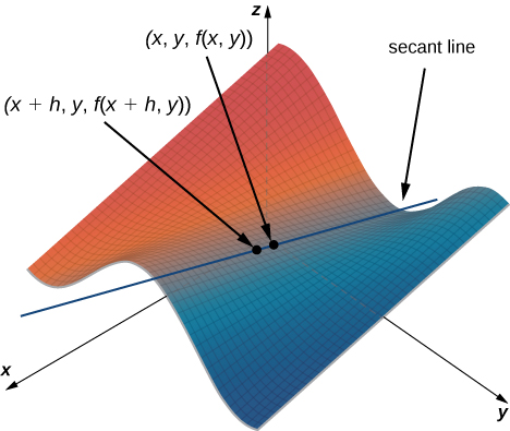
In Figure $\PageIndex{1}$, the value of $h$ is positive. If we graph $f(x,y)$ and $f(x+h,y)$ for an arbitrary point $(x,y),$ then the slope of the secant line passing through these two points is given by

$$\dfrac{f(x+h,y)−f(x,y)}{h}. \nonumber$$

This line is parallel to the $x$-axis. Therefore, the slope of the secant line represents an average rate of change of the function $f$ as we travel parallel to the $x$-axis. As $h$ approaches zero, the slope of the secant line approaches the slope of the tangent line.

If we choose to change $y$ instead of $x$ by the same incremental value $h$, then the secant line is parallel to the $y$-axis and so is the tangent line. Therefore, $∂f/∂x$ represents the slope of the tangent line passing through the point $(x,y,f(x,y))$ parallel to the $x$-axis and $∂f/∂y$ represents the slope of the tangent line passing through the point $(x,y,f(x,y))$ parallel to the $y$-axis. If we wish to find the slope of a tangent line passing through the same point in any other direction, then we need what are called directional derivatives.

We now return to the idea of contour maps, which we introduced in Functions of Several Variables. We can use a contour map to estimate partial derivatives of a function $g(x,y)$.

Example $\PageIndex{3}$: Partial Derivatives from a Contour Map

Use a contour map to estimate $∂g/∂x$ at the point $(\sqrt{5},0)$ for the function

$$g(x,y)=\sqrt{9−x^2−y^2}. \nonumber$$

Solution

Figure $\PageIndex{2}$ represents a contour map for the function $g(x,y)$.

Figure $\PageIndex{2}$: Contour map for the function $g(x,y)=\sqrt{9−x^2−y^2}$, using $c=0,1,2,$ and $3 (c=3$ corresponds to the origin).

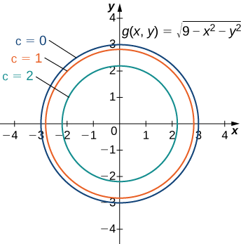
The inner circle on the contour map corresponds to $c=2$ and the next circle out corresponds to $c=1$. The first circle is given by the equation $2=\sqrt{9−x^2−y^2}$; the second circle is given by the equation $1=\sqrt{9−x^2−y^2}$. The first equation simplifies to $x^2+y^2=5$ and the second equation simplifies to $x^2+y^2=8.$ The $x$-intercept of the first circle is $(\sqrt{5},0)$ and the $x$-intercept of the second circle is $(2\sqrt{2},0)$. We can estimate the value of $∂g/∂x$ evaluated at the point $(\sqrt{5},0)$ using the slope formula:

$$\begin{align*} \left.\dfrac{∂g}{∂x}\right|_{(x,y) = (\sqrt{5},0)} &≈ \dfrac{g(\sqrt{5},0)−g(2\sqrt{2},0)}{\sqrt{5}−2\sqrt{2}} \\ &= \dfrac{2−1}{\sqrt{5}−2\sqrt{2}} \\ &=\dfrac{1}{\sqrt{5}−2\sqrt{2}} ≈−1.688. \end{align*}$$

To calculate the exact value of $∂g/∂x$ evaluated at the point $(\sqrt{5},0)$, we start by finding $∂g/∂x$ using the chain rule. First, we rewrite the function as

$$g(x,y)=\sqrt{9−x^2−y^2}=(9−x^2−y^2)^{1/2} \nonumber$$

and then differentiate with respect to $x$ while holding $y$ constant:

$$\begin{align*} \dfrac{∂g}{∂x} &=\dfrac{1}{2}(9−x^2−y^2)^{−1/2}(−2x) \\[4pt] &=−\dfrac{x}{\sqrt{9−x^2−y^2}}. \end{align*}$$

Next, we evaluate this expression using $x=\sqrt{5}$ and $y=0$:

$$\begin{align*} \dfrac{∂g}{∂x}∣_{(x,y) = (\sqrt{5},0)} &=−\dfrac{\sqrt{5}}{\sqrt{9−(\sqrt{5})^2−(0)^2}} \\[4pt] &=−\dfrac{\sqrt{5}}{\sqrt{4}} \\[4pt] &=−\dfrac{\sqrt{5}}{2} ≈−1.118. \end{align*} \nonumber$$

The estimate for the partial derivative corresponds to the slope of the secant line passing through the points $(\sqrt{5},0,g(\sqrt{5},0))$ and $(2\sqrt{2},0,g(2\sqrt{2},0))$. It represents an approximation to the slope of the tangent line to the surface through the point $(\sqrt{5},0,g(\sqrt{5},0)),$ which is parallel to the $x$-axis.

Exercise $\PageIndex{3}$

Use a contour map to estimate $∂f/∂y$ at point $(0,\sqrt{2})$ for the function

$$f(x,y)=x^2−y^2.\nonumber$$

Compare this with the exact answer.

Hint

Create a contour map for $f$ using values of $c$ from $−3$ to $3$. Which of these curves passes through point $(0,\sqrt{2})?$

Answer

Using the curves corresponding to $c=−2$ and $c=−3,$ we obtain

$$\begin{align*} \left. \dfrac{∂f}{∂y}\right|_{(x,y)=(0,\sqrt{2})} &≈\dfrac{f(0,\sqrt{3})−f(0,\sqrt{2})}{\sqrt{3}−\sqrt{2}} \\[4pt] &=\dfrac{−3−(−2)}{\sqrt{3}−\sqrt{2}}⋅\dfrac{\sqrt{3}+\sqrt{2}}{\sqrt{3}+\sqrt{2}} \\[4pt] &=−\sqrt{3}−\sqrt{2}≈−3.146. \end{align*}$$

The exact answer is

$$\left. \dfrac{∂f}{∂y} \right|_{(x,y)=(0,\sqrt{2})}=(−2y|_{(x,y)=(0,\sqrt{2})}=−2\sqrt{2}≈−2.828. \nonumber$$

Functions of More Than Two Variables

Suppose we have a function of three variables, such as $w=f(x,y,z).$ We can calculate partial derivatives of $w$ with respect to any of the independent variables, simply as extensions of the definitions for partial derivatives of functions of two variables.

Definition: Partial Derivatives

Let $f(x,y,z)$ be a function of three variables. Then, the partial derivative of $f$ with respect to $x$, written as $∂f/∂x,$ or $f_x,$ is defined to be

$$\dfrac{∂f}{∂x}=f_x(x,y,z)=\lim_{h→0}\dfrac{f(x+h,y,z)−f(x,y,z)}{h}. \label{PD2a}$$

The partial derivative of $f$ with respect to $y$, written as $∂f/∂y$, or $f_y$, is defined to be

$$\dfrac{∂f}{∂y}=f_y(x,y,z)=\lim_{k→0}\dfrac{f(x,y+k,z)−f(x,y,z)}{k.} \label{PD2b}$$

The partial derivative of $f$ with respect to $z$, written as $∂f/∂z$, or $f_z$, is defined to be

$$\dfrac{∂f}{∂z}=f_z(x,y,z)=\lim_{m→0}\dfrac{f(x,y,z+m)−f(x,y,z)}{m}. \label{PD2c}$$

We can calculate a partial derivative of a function of three variables using the same idea we used for a function of two variables. For example, if we have a function $f$ of $x,y$, and $z$, and we wish to calculate $∂f/∂x$, then we treat the other two independent variables as if they are constants, then differentiate with respect to $x$.

Example $\PageIndex{4}$: Calculating Partial Derivatives for a Function of Three Variables

Use the limit definition of partial derivatives to calculate $∂f/∂x$ for the function

$$f(x,y,z)=x^2−3xy+2y^2−4xz+5yz^2−12x+4y−3z. \nonumber$$

Then, find $∂f/∂y$ and $∂f/∂z$ by setting the other two variables constant and differentiating accordingly.

Solution:

We first calculate $∂f/∂x$ using Equation $\ref{PD2a}$, then we calculate the other two partial derivatives by holding the remaining variables constant. To use the equation to find $∂f/∂x$, we first need to calculate $f(x+h,y,z):$

$$\begin{align*} f(x+h,y,z) &=(x+h)^2−3(x+h)y+2y^2−4(x+h)z+5yz^2−12(x+h)+4y−3z \\[4pt] &=x^2+2xh+h^2−3xy−3xh+2y^2−4xz−4hz+5yz^2−12x−12h+4y−3z \end{align*} \nonumber$$

and recall that $f(x,y,z)=x^2−3xy+2y^2−4zx+5yz^2−12x+4y−3z.$ Next, we substitute these two expressions into the equation:

$$\begin{align*} \dfrac{∂f}{∂x} &=\lim_{h→0} \left[\dfrac{x^2+2xh+h^2−3xy−3hy+2y^2−4xz−4hz+5yz^2−12x−12h+4y−3zh−x^2−3xy+2y^2−4xz+5yz^2−12x+4y−3z}{h} \right] \\[4pt] &=\lim_{h→0} \left[\dfrac{2xh+h^2−3hy−4hz−12h}{h} \right] \\[4pt] &=\lim_{h→0} \left[\dfrac{h(2x+h−3y−4z−12)}{h} \right] \\[4pt] &=\lim_{h→0}(2x+h−3y−4z−12) \\[4pt] &=2x−3y−4z−12. \end{align*} \nonumber$$

Then we find $∂f/∂y$ by holding $x$ and $z$ constant. Therefore, any term that does not include the variable $y$ is constant, and its derivative is zero. We can apply the sum, difference, and power rules for functions of one variable:

$$\begin{align*} & \dfrac{∂}{∂y}\left[x^2−3xy+2y^2−4xz+5yz^2−12x+4y−3z\right] \\[4pt] &=\dfrac{∂}{∂y}[x^2]−\dfrac{∂}{∂y}[3xy]+\dfrac{∂}{∂y}[2y^2]−\dfrac{∂}{∂y}[4xz]+\dfrac{∂}{∂y}[5yz^2]−\dfrac{∂}{∂y}[12x]+\dfrac{∂}{∂y}[4y]−\dfrac{∂}{∂z}[3z] \\[4pt] &=0−3x+4y−0+5z^2−0+4−0 \\[4pt] &=−3x+4y+5z^2+4. \end{align*}$$

To calculate $∂f/∂z,$ we hold $x$ and $y$ constant and apply the sum, difference, and power rules for functions of one variable:

$$\begin{align*} & \dfrac{∂}{∂z}[x^2−3xy+2y^2−4xz+5yz^2−12x+4y−3z] \\[4pt] &=\dfrac{∂}{∂z}[x^2]−\dfrac{∂}{∂z}[3xy]+\dfrac{∂}{∂z}[2y^2]−\dfrac{∂}{∂z}[4xz]+\dfrac{∂}{∂z}[5yz^2]−\dfrac{∂}{∂z}[12x]+\dfrac{∂}{∂z}[4y]−\dfrac{∂}{∂z}[3z] \\[4pt] &=0−0+0−4x+10yz−0+0−3 \\[4pt] &=−4x+10yz−3 \end{align*}$$

Exercise $\PageIndex{4}$

Use the limit definition of partial derivatives to calculate $∂f/∂x$ for the function

$$f(x,y,z)=2x^2−4x^2y+2y^2+5xz^2−6x+3z−8.\nonumber$$

Then find $∂f/∂y$ and $∂f/∂z$ by setting the other two variables constant and differentiating accordingly.

Hint

Use the strategy in the preceding example.

Answer

$\dfrac{∂f}{∂x}=4x−8xy+5z^2−6,\dfrac{∂f}{∂y}=−4x^2+4y,\dfrac{∂f}{∂z}=10xz+3$

Example $\PageIndex{5}$: Calculating Partial Derivatives for a Function of Three Variables

Calculate the three partial derivatives of the following functions.

1. $f(x,y,z)=\dfrac{x^2y−4xz+y^2}{x−3yz}$
2. $g(x,y,z)=\sin(x^2y−z)+\cos(x^2−yz)$

Solution

In each case, treat all variables as constants except the one whose partial derivative you are calculating.

a.

$$\begin{align*} \dfrac{∂f}{∂x} &=\dfrac{∂}{∂x}\left[\dfrac{x^2y−4xz+y^2}{x−3yz}\right] \\[6pt] &=\dfrac{\dfrac{∂}{∂x}(x^2y−4xz+y^2)(x−3yz)−(x^2y−4xz+y^2)\dfrac{∂}{∂x}(x−3yz)}{(x−3yz)^2} \\[6pt] &=\dfrac{(2xy−4z)(x−3yz)−(x^2y−4xz+y^2)(1)}{(x−3yz)^2} \\[6pt] &=\dfrac{2x^2y−6xy^2z−4xz+12yz^2−x^2y+4xz−y^2}{(x−3yz)^2} \\[6pt] &=\dfrac{x^2y−6xy^2z−4xz+12yz^2+4xz−y^2}{(x−3yz)^2} \end{align*}$$

$$\begin{align*} \dfrac{∂f}{∂y} &=\dfrac{∂}{∂y}\left[\dfrac{x^2y−4xz+y^2}{x−3yz}\right] \\[6pt] &=\dfrac{\dfrac{∂}{∂y}(x^2y−4xz+y^2)(x−3yz)−(x^2y−4xz+y^2)\dfrac{∂}{∂y}(x−3yz)}{(x−3yz)^2} \\[6pt] &=\dfrac{(x^2+2y)(x−3yz)−(x^2y−4xz+y^2)(−3z)}{(x−3yz)^2} \\[6pt] &=\dfrac{x^3−3x^2yz+2xy−6y^2z+3x^2yz−12xz^2+3y^2z}{(x−3yz)^2} \\[6pt] &=\dfrac{x^3+2xy−3y^2z−12xz^2}{(x−3yz)^2} \end{align*}$$

$$\begin{align*} \dfrac{∂f}{∂z} &=\dfrac{∂}{∂z}\left[\dfrac{x^2y−4xz+y^2}{x−3yz}\right] \\[6pt] &=\dfrac{\dfrac{∂}{∂z}(x^2y−4xz+y^2)(x−3yz)−(x^2y−4xz+y^2)\dfrac{∂}{∂z}(x−3yz)}{(x−3yz)^2} \\[6pt] &=\dfrac{(−4x)(x−3yz)−(x^2y−4xz+y^2)(−3y)}{(x−3yz)^2} \\[6pt] &=\dfrac{−4x^2+12xyz+3x^2y^2−12xyz+3y^3}{(x−3yz)^2} \\[6pt] &=\dfrac{−4x^2+3x^2y^2+3y^3}{(x−3yz)^2} \end{align*}$$

b.

$$\begin{align*} \dfrac{∂f}{∂x} &=\dfrac{∂}{∂x} \left[\sin(x^2y−z)+\cos(x^2−yz) \right] \\[6pt] &=(\cos(x^2y−z))\dfrac{∂}{∂x}(x^2y−z)−(\sin(x^2−yz))\dfrac{∂}{∂x}(x^2−yz) \\[6pt] &=2xy\cos(x^2y−z)−2x\sin(x^2−yz) \end{align*}$$

$$\begin{align*} \dfrac{∂f}{∂y} &=\dfrac{∂}{∂y}[\sin(x^2y−z)+\cos(x^2−yz)] \\[6pt] &=(\cos(x^2y−z))\dfrac{∂}{∂y}(x^2y−z)−(\sin(x^2−yz))\dfrac{∂}{∂y}(x^2−yz) \\[6pt] &=x^2\cos(x^2y−z)+z\sin(x^2−yz) \end{align*}$$

$$\begin{align*} \dfrac{∂f}{∂z} &=\dfrac{∂}{∂z}[\sin(x^2y−z)+\cos(x^2−yz)] \\[6pt] &=(\cos(x^2y−z))\dfrac{∂}{∂z}(x^2y−z)−(\sin(x^2−yz))\dfrac{∂}{∂z}(x^2−yz) \\[6pt] &=−\cos(x^2y−z)+y\sin(x^2−yz) \end{align*} \nonumber$$

Exercise $\PageIndex{5}$

Calculate $∂f/∂x, ∂f/∂y,$ and $∂f/∂z$ for the function

$$f(x,y,z)=\sec(x^2y)−\tan(x^3yz^2). \nonumber$$

Hint

Use the strategy in the preceding example.

Answer

$\dfrac{∂f}{∂x}=2xy\sec(x^2y)\tan(x^2y)−3x^2yz^2\sec^2(x^3yz^2)$

$\dfrac{∂f}{∂y}=x^2\sec(x^2y)\tan(x^2y)−x^3z^2\sec^2(x^3yz^2)$

$\dfrac{∂f}{∂z}=−2x^3yz\sec^2(x^3yz^2)$

Higher-Order Partial Derivatives

Consider the function

$$f(x,y)=2x^3−4xy^2+5y^3−6xy+5x−4y+12. \nonumber$$

Its partial derivatives are

$$\dfrac{∂f}{∂x}=6x^2−4y^2−6y+5 \nonumber$$

and

$$\dfrac{∂f}{∂y}=−8xy+15y^2−6x−4. \nonumber$$

Each of these partial derivatives is a function of two variables, so we can calculate partial derivatives of these functions. Just as with derivatives of single-variable functions, we can call these second-order derivatives, third-order derivatives, and so on. In general, they are referred to as higher-order partial derivatives. There are four second-order partial derivatives for any function (provided they all exist):

$$\begin{align*} \dfrac{∂^2f}{∂x^2} &=\dfrac{∂}{∂x}\left[\dfrac{∂f}{∂x}\right] \\[4pt] \dfrac{∂^2f}{∂y∂x} &=\dfrac{∂}{∂y}\left[\dfrac{∂f}{∂x}\right] \\[4pt] \dfrac{∂^2f}{∂x∂y} &=\dfrac{∂}{∂x}\left[\dfrac{∂f}{∂y}\right] \\[4pt] \dfrac{∂^2f}{∂y^2} &=\dfrac{∂}{∂y}\left[\dfrac{∂f}{∂y}\right].\end{align*}$$

An alternative notation for each is $f_{xx},f_{xy},f_{yx},$ and $f_{yy}$, respectively. Higher-order partial derivatives calculated with respect to different variables, such as $f_{xy}$ and $f_{yx}$, are commonly called mixed partial derivatives.

Example $\PageIndex{6}$: Calculating Second Partial Derivatives

Calculate all four second partial derivatives for the function

$$f(x,y)=xe^{−3y}+\sin(2x−5y).\label{Ex6e1}$$

Solution:

To calculate $\dfrac{∂^2f}{∂x^2}$ and $\dfrac{∂^2f}{∂y∂x}$, we first calculate $∂f/∂x$:

$$\dfrac{∂f}{∂x}=e^{−3y}+2\cos(2x−5y). \label{Ex6e2}$$

To calculate $\dfrac{∂^2f}{∂x^2}$, differentiate $∂f/∂x$ (Equation $\ref{Ex6e2}$) with respect to $x$:

$$\begin{align*} \dfrac{∂^2f}{∂x^2} &=\dfrac{∂}{∂x}\left[\dfrac{∂f}{∂x}\right] \\[6pt] &=\dfrac{∂}{∂x}[e^{−3y}+2\cos(2x−5y)] \\[6pt] &=−4\sin(2x−5y). \end{align*} \nonumber$$

To calculate $\dfrac{∂^2f}{∂y∂x}$, differentiate $∂f/∂x$ (Equation $\ref{Ex6e2}$) with respect to $y$:

$$\begin{align*} \dfrac{∂^2f}{∂y\,∂x} &=\dfrac{∂}{∂y}\left[\dfrac{∂f}{∂x}\right] \\[6pt] &=\dfrac{∂}{∂y}[e^{−3y}+2\cos(2x−5y)] \\[6pt] &=−3e^{−3y}+10\sin(2x−5y). \end{align*} \nonumber$$

To calculate $\dfrac{∂^2f}{∂x∂y}$ and $\dfrac{∂^2f}{∂y^2}$, first calculate $∂f/∂y$:

$$\dfrac{∂f}{∂y}=−3xe^{−3y}−5\cos(2x−5y). \label{Ex6e5}$$

To calculate $\dfrac{∂^2f}{∂x∂y}$, differentiate $∂f/∂y$ (Equation $\ref{Ex6e5}$) with respect to $x$:

$$\begin{align*} \dfrac{∂^2f}{∂x∂y} &=\dfrac{∂}{∂x} \left[\dfrac{∂f}{∂y} \right] \\[6pt] &=\dfrac{∂}{∂x}[−3xe^{−3y}−5\cos(2x−5y)] \\[6pt] &=−3e^{−3y}+10\sin(2x−5y). \end{align*} \nonumber$$

To calculate $\dfrac{∂^2f}{∂y^2}$, differentiate $∂f/∂y$ (Equation $\ref{Ex6e5}$) with respect to $y$:

$$\begin{align*} \dfrac{∂^2f}{∂y^2} &=\dfrac{∂}{∂y}\left[\dfrac{∂f}{∂y}\right] \\[6pt] &=\dfrac{∂}{∂y}[−3xe^{−3y}−5\cos(2x−5y)] \\[6pt] &=9xe^{−3y}−25\sin(2x−5y). \end{align*} \nonumber$$

Exercise $\PageIndex{6}$

Calculate all four second partial derivatives for the function

$$f(x,y)=\sin(3x−2y)+\cos(x+4y).\nonumber$$

Hint

Follow the same steps as in the previous example.

Answer

$\dfrac{∂^2f}{∂x^2}=−9\sin(3x−2y)−\cos(x+4y)$

$\dfrac{∂^2f}{∂y∂x}=6\sin(3x−2y)−4\cos(x+4y)$

$\dfrac{∂^2f}{∂x∂y}=6\sin(3x−2y)−4\cos(x+4y)$

$\dfrac{∂^2f}{∂y^2}=−4\sin(3x−2y)−16\cos(x+4y)$

At this point we should notice that, in both Example $\PageIndex{6}$ and the checkpoint, it was true that $\dfrac{∂^2f}{∂y∂x}=\dfrac{∂^2f}{∂x∂y}$. Under certain conditions, this is always true. In fact, it is a direct consequence of the following theorem.

Theorem $\PageIndex{1}$: Equality of Mixed Partial Derivatives (Clairaut’s Theorem)

Suppose that $f(x,y)$ is defined on an open disk $D$ that contains the point $(a,b)$. If the functions $f_{xy}$ and $f_{yx}$ are continuous on $D$, then $f_{xy}(a,b)=f_{yx}(a,b)$.

Clairaut’s theorem guarantees that as long as mixed second-order derivatives are continuous, the order in which we choose to differentiate the functions (i.e., which variable goes first, then second, and so on) does not matter. It can be extended to higher-order derivatives as well. The proof of Clairaut’s theorem can be found in most advanced calculus books.

Two other second-order partial derivatives can be calculated for any function $f(x,y).$ The partial derivative $f_{xx}$ is equal to the partial derivative of $f_x$ with respect to $x$, and $f_{yy}$ is equal to the partial derivative of $f_y$ with respect to $y$.

Partial Differential Equations

Previously, we studied differential equations in which the unknown function had one independent variable. A partial differential equation is an equation that involves an unknown function of more than one independent variable and one or more of its partial derivatives. Examples of partial differential equations are

$$\underset{\text{heat equation in two dimensions}}{u_t=c^2(u_{xx}+u_{yy})} \nonumber$$

$$\underset{\text{wave equation in two dimensions}}{u_{tt}=c^2(u_{xx}+u_{yy})} \nonumber$$

$$\underset{\text{Laplace’s equation in two dimensions}} {u_{xx}+u_{yy}=0} \nonumber$$

In the heat and wave equations, the unknown function $u$ has three independent variables: $t$, $x$, and $y$ with $c$ is an arbitrary constant. The independent variables $x$ and $y$ are considered to be spatial variables, and the variable $t$ represents time. In Laplace’s equation, the unknown function $u$ has two independent variables $x$ and $y$.

Example $\PageIndex{7}$: A Solution to the Wave Equation

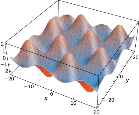
Verify that

$$u(x,y,t)=5\sin(3πx)\sin(4πy)\cos(10πt) \nonumber$$

is a solution to the wave equation

$$u_{tt}=4(u_{xx}+u_{yy}). \label{Ex7Eq2}$$

Solution

First, we calculate $u_{tt},u_{xx},$ and $u_{yy}:$

$$\begin{align*} u_{tt}(x,y,t) &=\dfrac{∂}{∂t}\left[\dfrac{∂u}{∂t}\right] \\[6pt] &=\dfrac{∂}{∂t}[5\sin(3πx)\sin(4πy)(−10π\sin(10πt))] \\[6pt] &= \dfrac{∂}{∂t} \left[−50π\sin(3πx)\sin(4πy)\sin(10πt)\right] \\[6pt] &=−500π^2\sin(3πx)\sin(4πy)\cos(10πt) \end{align*}$$

$$\begin{align*} u_{xx}(x,y,t) &=\dfrac{∂}{∂x} \left[\dfrac{∂u}{∂x}\right] \\[6pt] &=\dfrac{∂}{∂x}\left[15π\cos(3πx)\sin(4πy)\cos(10πt)\right] \\[6pt] &=−45π^2\sin(3πx)\sin(4πy)\cos(10πt) \end{align*}$$

$$\begin{align*} u_{yy}(x,y,t) &=\dfrac{∂}{∂y} \left[\dfrac{∂u}{∂y} \right] \\[6pt] &=\dfrac{∂}{∂y}\left[5\sin(3πx)(4π\cos(4πy))\cos(10πt)\right] \\[6pt] &=\dfrac{∂}{∂y}\left[20π\sin(3πx)\cos(4πy)\cos(10πt)\right] \\[6pt] &=−80π^2\sin(3πx)\sin(4πy)\cos(10πt). \end{align*} \nonumber$$

Next, we substitute each of these into the right-hand side of Equation $\ref{Ex7Eq2}$ and simplify:

$$\begin{align*} 4(u_{xx}+u_{yy}) &=4(−45π^2\sin(3πx)\sin(4πy)\cos(10πt)+−80π^2\sin(3πx)\sin(4πy)\cos(10πt)) \\[6pt] &=4(−125π^2\sin(3πx)\sin(4πy)\cos(10πt)) \\[6pt] &=−500π^2\sin(3πx)\sin(4πy)\cos(10πt) \\[6pt] &=u_{tt}. \end{align*}$$

This verifies the solution.

Exercise $\PageIndex{7}$: A Solution to the Heat Equation

Verify that

$$u(x,y,t)=2\sin \left(\dfrac{x}{3} \right)\sin\left(\dfrac{y}{4} \right)e^{−25t/16} \nonumber$$

is a solution to the heat equation

$$u_t=9(u_{xx}+u_{yy}). \nonumber$$

Hint

Calculate the partial derivatives and substitute into the right-hand side.

Answer

TBA

Since the solution to the two-dimensional heat equation is a function of three variables, it is not easy to create a visual representation of the solution. We can graph the solution for fixed values of $t,$ which amounts to snapshots of the heat distributions at fixed times. These snapshots show how the heat is distributed over a two-dimensional surface as time progresses. The graph of the preceding solution at time $t=0$ appears in Figure $\PageIndex{3}$. As time progresses, the extremes level out, approaching zero as $t$ approaches infinity.

Figure $\PageIndex{3}$

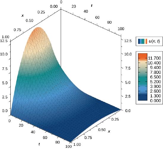
If we consider the heat equation in one dimension, then it is possible to graph the solution over time. The heat equation in one dimension becomes

$$u_t=c^2u_{xx}, \nonumber$$

where $c^2$ represents the thermal diffusivity of the material in question. A solution of this differential equation can be written in the form

$$u_m(x,t)=e^{−π^2m^2c^2t}\sin(mπx) \nonumber$$

where $m$ is any positive integer. A graph of this solution using $m=1$ appears in Figure $\PageIndex{4}$, where the initial temperature distribution over a wire of length $1$ is given by $u(x,0)=\sin πx.$ Notice that as time progresses, the wire cools off. This is seen because, from left to right, the highest temperature (which occurs in the middle of the wire) decreases and changes color from red to blue.

Figure $\PageIndex{4}$: Graph of a solution of the heat equation in one dimension over time.

Lord Kelvin and the Age of Earth

During the late 1800s, the scientists of the new field of geology were coming to the conclusion that Earth must be “millions and millions” of years old. At about the same time, Charles Darwin had published his treatise on evolution. Darwin’s view was that evolution needed many millions of years to take place, and he made a bold claim that the Weald chalk fields, where important fossils were found, were the result of $300$ million years of erosion.

Figure $\PageIndex{5}$: (a) William Thomson (Lord Kelvin), 1824-1907, was a British physicist and electrical engineer; (b) Kelvin used the heat diffusion equation to estimate the age of Earth (credit: modification of work by NASA).

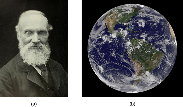
At that time, eminent physicist William Thomson (Lord Kelvin) used an important partial differential equation, known as the heat diffusion equation, to estimate the age of Earth by determining how long it would take Earth to cool from molten rock to what we had at that time. His conclusion was a range of 20 to 400 million years, but most likely about 50 million years. For many decades, the proclamations of this irrefutable icon of science did not sit well with geologists or with Darwin.

• Read Kelvin’s paper on estimating the age of the Earth.

Kelvin made reasonable assumptions based on what was known in his time, but he also made several assumptions that turned out to be wrong. One incorrect assumption was that Earth is solid and that the cooling was therefore via conduction only, hence justifying the use of the diffusion equation. But the most serious error was a forgivable one—omission of the fact that Earth contains radioactive elements that continually supply heat beneath Earth’s mantle. The discovery of radioactivity came near the end of Kelvin’s life and he acknowledged that his calculation would have to be modified.

Kelvin used the simple one-dimensional model applied only to Earth’s outer shell, and derived the age from graphs and the roughly known temperature gradient near Earth’s surface. Let’s take a look at a more appropriate version of the diffusion equation in radial coordinates, which has the form

$$\dfrac{∂T}{∂t}=K\left[\dfrac{∂^2T}{∂^2r}+\dfrac{2}{r}\dfrac{∂T}{∂r}\right] \label{kelvin1}$$.

Here, $T(r,t)$ is temperature as a function of $r$ (measured from the center of Earth) and time $t. K$ is the heat conductivity—for molten rock, in this case. The standard method of solving such a partial differential equation is by separation of variables, where we express the solution as the product of functions containing each variable separately. In this case, we would write the temperature as

$$T(r,t)=R(r)f(t). \nonumber$$

1. Substitute this form into Equation $\ref{kelvin1}$ and, noting that $f(t)$ is constant with respect to distance $(r)$ and $R(r)$ is constant with respect to time $(t)$, show that $$\dfrac{1}{f}\dfrac{∂f}{∂t}=\dfrac{K}{R}\left[\dfrac{∂^2R}{∂r^2}+\dfrac{2}{r}\dfrac{∂R}{∂r}\right]. \nonumber$$
2. This equation represents the separation of variables we want. The left-hand side is only a function of $t$ and the right-hand side is only a function of $r$, and they must be equal for all values of $r$ and $t$. Therefore, they both must be equal to a constant. Let’s call that constant $−λ^2$. (The convenience of this choice is seen on substitution.) So, we have $$\dfrac{1}{f}\dfrac{∂f}{∂t}=−λ^2 \text{and} \dfrac{K}{R}\left[\dfrac{∂^2R}{∂r^2}+\dfrac{2}{r}\dfrac{∂R}{∂r}\right]=−λ^2. \nonumber$$
3. Now, we can verify through direct substitution for each equation that the solutions are $f(t)=Ae^{−λ^2t}$ and $R(r)=B\left(\dfrac{\sin αr}{r}\right)+C\left(\dfrac{\cos αr}{r}\right)$, where $α=λ/\sqrt{K}$. Note that $f(t)=Ae^{+λn^2t}$ is also a valid solution, so we could have chosen $+λ^2$for our constant. Can you see why it would not be valid for this case as time increases?
4. Let’s now apply boundary conditions.
   1. The temperature must be finite at the center of Earth, $r=0$. Which of the two constants, $B$ or $C$, must therefore be zero to keep $R$ finite at $r=0$? (Recall that $\sin(αr)/r→α=$ as $r→0$, but $\cos(αr)/r$ behaves very differently.)
   2. Kelvin argued that when magma reaches Earth’s surface, it cools very rapidly. A person can often touch the surface within weeks of the flow. Therefore, the surface reached a moderate temperature very early and remained nearly constant at a surface temperature $T_s$. For simplicity, let’s set $T=0$ at $r=R_E$ and find α such that this is the temperature there for all time $t$. (Kelvin took the value to be $300K≈80°F$. We can add this $300K$ constant to our solution later.) For this to be true, the sine argument must be zero at $r=R_E$. Note that α has an infinite series of values that satisfies this condition. Each value of $α$ represents a valid solution (each with its own value for $A$). The total or general solution is the sum of all these solutions.
   3. At $t=0,$ we assume that all of Earth was at an initial hot temperature $T_0$ (Kelvin took this to be about $7000K$.) The application of this boundary condition involves the more advanced application of Fourier coefficients. As noted in part b. each value of $α_n$ represents a valid solution, and the general solution is a sum of all these solutions. This results in a series solution: $$T(r,t)=\left(\dfrac{T_0R_E}{π}\right)\sum_n\dfrac{(−1)^{n−1}}{n}e^{−λn^2t}\dfrac{\sin(α_nr)}{r} \nonumber$$ where $\; α_n=nπ/R_E$.

Note how the values of $α_n$ come from the boundary condition applied in part b. The term $\dfrac{−1^{n−1}}{n}$ is the constant $A_n$ for each term in the series, determined from applying the Fourier method. Letting $β=\dfrac{π}{R_E}$, examine the first few terms of this solution shown here and note how $λ^2$ in the exponential causes the higher terms to decrease quickly as time progresses:

$$T(r,t)=\dfrac{T_0R_E}{πr}\left(e^{−Kβ^2t}(\sinβr)−\dfrac{1}{2}e^{−4Kβ^2t}(\sin2βr)+\dfrac{1}{3}e^{−9Kβ^2t}(\sin3βr)−\dfrac{1}{4}e^{−16Kβ^2t}(\sin4βr)+\dfrac{1}{5}e^{−25Kβ^2t}(\sin5βr)...\right). \nonumber$$

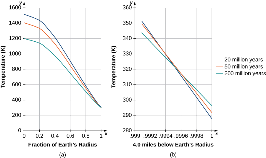
Near time $t=0,$ many terms of the solution are needed for accuracy. Inserting values for the conductivity $K$ and $β=π/R_E$ for time approaching merely thousands of years, only the first few terms make a significant contribution. Kelvin only needed to look at the solution near Earth’s surface (Figure $\PageIndex{6}$) and, after a long time, determine what time best yielded the estimated temperature gradient known during his era ( $1°F$ increase per $50ft$). He simply chose a range of times with a gradient close to this value. In Figure $\PageIndex{6}$, the solutions are plotted and scaled, with the $300−K$ surface temperature added. Note that the center of Earth would be relatively cool. At the time, it was thought Earth must be solid.

Figure $\PageIndex{6}$: Temperature versus radial distance from the center of Earth. (a) Kelvin’s results, plotted to scale. (b) A close-up of the results at a depth of $4.0$ miles below Earth’s surface.

Epilog

On May 20, 1904, physicist Ernest Rutherford spoke at the Royal Institution to announce a revised calculation that included the contribution of radioactivity as a source of Earth’s heat. In Rutherford’s own words:

“I came into the room, which was half-dark, and presently spotted Lord Kelvin in the audience, and realized that I was in for trouble at the last part of my speech dealing with the age of the Earth, where my views conflicted with his. To my relief, Kelvin fell fast asleep, but as I came to the important point, I saw the old bird sit up, open an eye and cock a baleful glance at me.

Then a sudden inspiration came, and I said Lord Kelvin had limited the age of the Earth, provided no new source [of heat] was discovered. That prophetic utterance referred to what we are now considering tonight, radium! Behold! The old boy beamed upon me.”

Rutherford calculated an age for Earth of about 500 million years. Today’s accepted value of Earth’s age is about 4.6 billion years.

Key Concepts

• A partial derivative is a derivative involving a function of more than one independent variable.
• To calculate a partial derivative with respect to a given variable, treat all the other variables as constants and use the usual differentiation rules.
• Higher-order partial derivatives can be calculated in the same way as higher-order derivatives.

Key Equations

Partial derivative of $f$ with respect to $x$ $$\dfrac{∂f}{∂x}=\displaystyle{\lim_{h→0}\dfrac{f(x+h,y)−f(x,y)}{h}} \nonumber$$

Partial derivative of $f$ with respect to $y$ $$\dfrac{∂f}{∂y}=\displaystyle{\lim_{k→0}\dfrac{f(x,y+k)−f(x,y)}{k}} \nonumber$$

Glossary

higher-order partial derivatives

second-order or higher partial derivatives, regardless of whether they are mixed partial derivatives

mixed partial derivatives

second-order or higher partial derivatives, in which at least two of the differentiations are with respect to different variables

partial derivative

a derivative of a function of more than one independent variable in which all the variables but one are held constant

partial differential equation

an equation that involves an unknown function of more than one independent variable and one or more of its partial derivatives