2.3: Basic Differentiation Rules

The derivative is a powerful tool but is admittedly awkward given its reliance on limits. Fortunately, one thing mathematicians are good at is abstraction. For instance, instead of continually finding derivatives at a point, we abstracted and found the derivative function.

Let's practice abstraction on linear functions, \(y=mx+b\). What is \(y^\prime\)? Without limits, recognize that linear function are characterized by being functions with a constant rate of change (the slope). The derivative, \(y^\prime\), gives the instantaneous rate of change; with a linear function, this is constant, \(m\). Thus \(y^\prime =m\).

Let's abstract once more. Let's find the derivative of the general quadratic function, \(f(x) = ax^2+bx+c\). Using the definition of the derivative, we have:

\[\begin{align*}f^\prime (x) &= \lim_{h\to 0}\frac{a(x+h)^2+b(x+h)+c-(ax^2+bx+c)}{h} \\ &= \lim_{h\to 0} \frac{ah^2+2ahx+bh}{h} \\ &= \lim_{h\to 0} ah+2ax+b\\ &= 2ax+b. \end{align*}\]

So if \(y = 6x^2+11x-13\), we can immediately compute \(y^\prime = 12x+11\).

In this section (and in some sections to follow) we will learn some of what mathematicians have already discovered about the derivatives of certain functions and how derivatives interact with arithmetic operations. We start with a theorem.

Theorem 12: Derivatives of Common Functions

This theorem starts by stating an intuitive fact: constant functions have no rate of change as they are constant. Therefore their derivative is 0 (they change at the rate of 0). The theorem then states some fairly amazing things. The Power Rule states that the derivatives of Power Functions (of the form \(y=x^n\)) are very straightforward: multiply by the power, then subtract 1 from the power. We see something incredible about the function \(y=e^x\): it is its own derivative. We also see a new connection between the sine and cosine functions.

One special case of the Power Rule is when \(n=1\), i.e., when \(f(x) = x\). What is \(f^\prime (x)\)? According to the Power Rule, \[f^\prime (x) = \frac{d}{dx}\big(x\big) = \frac{d}{dx}\big(x^1\big) = 1\cdot x^0 = 1.\]In words, we are asking "At what rate does \(f\) change with respect to \(x\)?'' Since \(f\) is \(x\), we are asking "At what rate does \(x\) change with respect to \(x\)?'' The answer is: 1. They change at the same rate.

Let's practice using this theorem.

Example 46: Using Theorem 12 to find, and use, derivatives

Let \(f(x)=x^3\).

1. Find \(f^\prime (x)\).
2. Find the equation of the line tangent to the graph of \(f\) at \(x=-1\).
3. Use the tangent line to approximate \((-1.1)^3\).
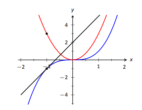
4. Sketch \(f\), \(f^\prime \) and the found tangent line on the same axis.

Solution

1. The Power Rule states that if \(f(x) = x^3\), then \(f^\prime (x) = 3x^2\).
2. To find the equation of the line tangent to the graph of \(f\) at \(x=-1\), we need a point and the slope. The point is \((-1,f(-1)) = (-1, -1)\). The slope is \(f^\prime (-1)= 3\). Thus the tangent line has equation \(y = 3(x-(-1))+(-1) = 3x+2\).
3. We can use the tangent line to approximate \((-1.1)^3\) as \(-1.1\) is close to \(-1\). We have \[(-1.1)^3 \approx 3(-1.1)+2 = -1.3.\]
   We can easily find the actual answer; \((-1.1)^3 = -1.331\).
4. See Figure 2.14.

Figure 2.14: A graph of \(f(x)=x^3\), along with its derivatives \(f^\prime (x)=3x^2\) and its tangent line at \(x=-1\).

Theorem 12 gives useful information, but we will need much more. For instance, using the theorem, we can easily find the derivative of \(y=x^3\), but it does not tell how to compute the derivative of \(y=2x^3\), \(y=x^3+\sin x\) nor \(y=x^3\sin x\). The following theorem helps with the first two of these examples (the third is answered in the next section).

Theorem 13: Properties of the Derivative

Let \(f\) and \(g\) be differentiable on an open interval \(I\) and let \(c\) be a real number. Then:

1. Sum/Difference Rule:
   \( \frac{d}{dx}\Big(f(x) \pm g(x)\Big) = \frac{d}{dx}\Big(f(x)\Big) \pm \frac{d}{dx}\Big(g(x)\Big) = f^\prime (x)\pm g^\prime (x)\)
2. Constant Multiple Rule:
   \(\frac{d}{dx}\Big(c\cdot f(x)\Big) = c \cdot \frac{d}{dx}\Big(f(x)\Big) = c\cdot f^\prime (x)\).

Theorem 13 allows us to find the derivatives of a wide variety of functions. It can be used in conjunction with the Power Rule to find the derivatives of any polynomial. Recall in Example 36 that we found, using the limit definition, the derivative of \(f(x) = 3x^2+5x-7\). We can now find its derivative without expressly using limits:

\[\begin{align*}\frac{d}{dx}\Big(3x^2+5x+7\Big) &= 3\frac{d}{dx}\Big(x^2\Big) + 5\frac{d}{dx}\Big(x\Big) + \frac{d}{dx}\Big(7\Big) \\ &= 3\cdot 2x+5\cdot 1+ 0\\ &= 6x+5. \end{align*}\]

We were a bit pedantic here, showing every step. Normally we would do all the arithmetic and steps in our head and readily find \( \frac{d}{dx}\Big(3x^2+5x+7\Big) = 6x+5.\)

Example 47: Using the tangent line to approximate a function value

Let \(f(x) = \sin x + 2x+1\). Approximate \(f(3)\) using an appropriate tangent line.

Solution

This problem is intentionally ambiguous; we are to approximate using an appropriate tangent line. How good of an approximation are we seeking? What does appropriate mean?

In the "real world,'' people solving problems deal with these issues all time. One must make a judgment using whatever seems reasonable. In this example, the actual answer is \(f(3) = \sin 3 + 7\), where the real problem spot is \(\sin 3\). What is \(\sin 3\)?

Since \(3\) is close to \(\pi\), we can assume \(\sin 3\approx \sin \pi = 0\). Thus one guess is \(f(3) \approx 7\). Can we do better? Let's use a tangent line as instructed and examine the results; it seems best to find the tangent line at \(x=\pi\).

Using Theorem 12 we find \(f^\prime (x) = \cos x + 2\). The slope of the tangent line is thus \(f^\prime (\pi) = \cos \pi + 2 =1\). Also, \(f(\pi) = 2\pi+1 \approx 7.28\). So the tangent line to the graph of \(f\) at \(x=\pi\) is \(y=1(x-\pi)+ 2\pi+1 =x+\pi+1 \approx x+4.14\). Evaluated at \(x=3\), our tangent line gives \(y=3+4.14 = 7.14\). Using the tangent line, our final approximation is that \(f(3) \approx 7.14\).

Using a calculator, we get an answer accurate to 4 places after the decimal: \(f(3) = 7.1411\). Our initial guess was \(7\); our tangent line approximation was more accurate, at \(7.14\).

The point is not "Here's a cool way to do some math without a calculator.'' Sure, that might be handy sometime, but your phone could probably give you the answer. Rather, the point is to say that tangent lines are a good way of approximating, and many scientists, engineers and mathematicians often face problems too hard to solve directly. So they approximate.

Higher Order Derivatives

The derivative of a function \(f\) is itself a function, therefore we can take its derivative. The following definition gives a name to this concept and introduces its notation.

Definition 11: Higher Order Derivatives

Let \(y=f(x)\) be a differentiable function on \(I\).

1. The second derivative of \(f\) is:

\[ f^{\prime\prime}(x) = \frac{d}{dx}\Big(f^\prime (x)\Big) = \frac{d}{dx}\left(\frac{dy}{dx}\right) = \frac{d^2y}{dx^2}=y^{\prime\prime} .\]

1. The third derivative of \(f\) is:

\[ f^{\prime\prime\prime} (x) = \frac{d}{dx}\Big(f^{\prime\prime}(x)\Big) = \frac{d}{dx}\left(\frac{d^2y}{dx^2}\right) = \frac{d^3y}{dx^3}=y^{\prime\prime\prime} .\]

1. The \(n^{\text{th}}\) derivative} of \(f\) is:

\[ f^{(n)}(x) = \frac{d}{dx}\left(f^{(n-1)}(x)\right) = \frac{d}{dx}\left(\frac{d^{n-1}y}{dx^{n-1}}\right) = \frac{d^ny}{dx^n}=y^{(n)}.\]

In general, when finding the fourth derivative and on, we resort to the \(f^{(4)}(x)\) notation, not \(f^{\prime\prime\prime\prime}(x)\); after a while, too many ticks is too confusing.

Let's practice using this new concept.

Example 48: Finding higher order derivatives

Find the first four derivatives of the following functions:

1. \(f(x) = 4x^2\)
2. \(f(x) = \sin x\)
3. \(f(x) = 5e^x\)

Solution

1. Using the Power and Constant Multiple Rules, we have: \(f^\prime (x) = 8x\). Continuing on, we have\[f^{\prime\prime}(x) = \frac{d}{dx}\big(8x\big) = 8;\qquad f^{\prime\prime\prime} (x) = 0;\qquad f^{(4)}(x) = 0.\]Notice how all successive derivatives will also be 0.
2. We employ Theorem 12 repeatedly.\[f^\prime (x) = \cos x;\qquad f^{\prime\prime}(x) = -\sin x;\qquad f^{\prime\prime\prime}(x) = -\cos x;\qquad f^{(4)}(x) = \sin x.\]Note how we have come right back to \(f(x)\) again. (Can you quickly figure what \(f\,^{(23)}(x)\) is?)
3. Employing Theorem 12 and the Constant Multiple Rule, we can see that \[f^\prime (x) = f^{\prime\prime}(x) = f^{\prime\prime\prime}(x) = f^{(4)}(x) = 5e^x.\]

Interpreting Higher Order Derivatives

What do higher order derivatives mean? What is the practical interpretation? Our first answer is a bit wordy, but is technically correct and beneficial to understand. That is,

\[\text{The second derivative of a function \(f\) is the rate of change of the rate of change of \(f\).}\]

One way to grasp this concept is to let \(f\) describe a position function. Then, as stated in Key Idea 1, \(f^\prime \) describes the rate of position change: velocity. We now consider \(f^{\prime\prime}\), which describes the rate of velocity change. Sports car enthusiasts talk of how fast a car can go from 0 to 60 mph; they are bragging about the acceleration of the car.

We started this chapter with amusement--park riders free--falling with position function \(f(t) = -16t^2+150\). It is easy to compute \(f^\prime (t)=-32t\) ft/s and \(f^{\prime\prime}(t) = -32\) (ft/s)/s. We may recognize this latter constant; it is the acceleration due to gravity. In keeping with the unit notation introduced in the previous section, we say the units are "feet per second per second.'' This is usually shortened to "feet per second squared,'' written as "ft/s\(^2\).''

It can be difficult to consider the meaning of the third, and higher order, derivatives. The third derivative is "the rate of change of the rate of change of the rate of change of \(f\).'' That is essentially meaningless to the uninitiated. In the context of our position/velocity/acceleration example, the third derivative is the "rate of change of acceleration,'' commonly referred to as "jerk.''

Make no mistake: higher order derivatives have great importance even if their practical interpretations are hard (or "impossible'') to understand. The mathematical topic of series makes extensive use of higher order derivatives.