11.3: The Calculus of Motion

A common use of vector--valued functions is to describe the motion of an object in the plane or in space. A position function \(\vecs r(t)\) gives the position of an object at time \(t\). This section explores how derivatives and integrals are used to study the motion described by such a function.

Definition 73: Velocity, Speed and Acceleration

Let \(\vecs r(t)\) be a position function in \(\mathbb{R}^2\) or \(\mathbb{R}^3\).

• Velocity, denoted \(\vecs v(t)\), is the instantaneous rate of position change; that is,

\[\vecs v(t) = \vecs r^\prime (t).\]

• Speed is the magnitude of velocity,

\[ \text{speed} = \norm{\vecs v(t)}.\]

• Acceleration, denoted \(\vecs a(t)\), is the instantaneous rate of velocity change; that is,

\[\vecs a(t) = \vecs v\,'(t) = \vecs r^{\prime\prime}(t).\]

Example \(\PageIndex{1}\): Finding velocity and acceleration

An object is moving with position function \(\vecs r(t) = \langle t^2-t,t^2+t\rangle\), \(-3\leq t\leq 3\), where distances are measured in feet and time is measured in seconds.

1. Find \(\vecs v (t)\) and \(\vecs a (t)\).
2. Sketch \(\vecs r (t)\); plot \(\vecs v(-1)\), \(\vecs a(-1)\), \(\vecs v(1)\) and \(\vecs a(1)\), each with their initial point at their corresponding point on the graph of \(\vecs r (t)\).
3. When is the object's speed minimized?

Solution

1. Taking derivatives, we find \[\vecs v (t) = \vecs r^\prime (t) =\langle 2t-1,2t+1\rangle \nonumber\] and \[\quad \vecs a (t) = \vecs r^{\prime\prime}(t) = \langle 2,2\rangle. \nonumber\] Note that acceleration is constant.
   
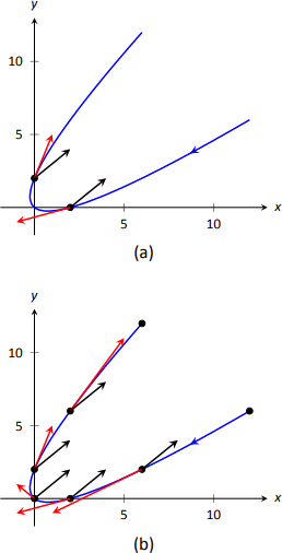
2. \(\vecs v(-1) = \langle -3,-1\rangle\), \(\vecs a(-1) = \langle 2,2\rangle\); \(\vecs v(1) = \langle 1,3\rangle\), \(\vecs a(1) = \langle 2,2\rangle\). These are plotted with \(\vecs r (t)\) in Figure \(\PageIndex{1a}\).
   We can think of acceleration as "pulling'' the velocity vector in a certain direction. At \(t=-1\), the velocity vector points down and to the left; at \(t=1\), the velocity vector has been pulled in the \(\langle 2,2\rangle\) direction and is now pointing up and to the right. In Figure 11.15(b) we plot more velocity/acceleration vectors, making more clear the effect acceleration has on velocity.
   Since \(\vecs a (t)\) is constant in this example, as \(t\) grows large \(\vecs v (t)\) becomes almost parallel to \(\vecs a (t)\). For instance, when \(t=10\), \(\vecs v(10) = \langle 19,21\rangle\), which is nearly parallel to \(\langle 2,2\rangle\).
3. The object's speed is given by \[\norm{\vecs v (t)} = \sqrt{(2t-1)^2+(2t+1)^2} =\sqrt{8t^2+2}.\] To find the minimal speed, we could apply calculus techniques (such as set the derivative equal to 0 and solve for \(t\), etc.) but we can find it by inspection. Inside the square root we have a quadratic which is minimized when \(t=0\). Thus the speed is minimized at \(t=0\), with a speed of \(\sqrt{2}\) ft/s.
   
   The graph in Figure \(\PageIndex{1b}\) also implies speed is minimized here. The filled dots on the graph are located at integer values of \(t\) between \(-3\) and 3. Dots that are far apart imply the object traveled a far distance in 1 second, indicating high speed; dots that are close together imply the object did not travel far in 1 second, indicating a low speed. The dots are closest together near \(t=0\), implying the speed is minimized near that value.

Figure \(\PageIndex{1}\): Graphing the position, velocity and acceleration of an object in Example 11.3.1

Example \(\PageIndex{2}\): Analyzing Motion

Two objects follow an identical path at different rates on \([-1,1]\). The position function for Object 1 is \(\vecs r_1(t) = \langle t, t^2\rangle\); the position function for Object 2 is \(\vecs r_2(t) = \langle t^3, t^6\rangle\), where distances are measured in feet and time is measured in seconds. Compare the velocity, speed and acceleration of the two objects on the path.

Solution

We begin by computing the velocity and acceleration function for each object:

\[\begin{align*}
\vecs v_1(t) &= \langle 1,2t\rangle & \vecs v_2(t) &= \langle 3t^2,6t^5\rangle \\[4pt]
\vecs a_1(t) &= \langle 0,2\rangle & \vecs a_2(t) &=\langle 6t,30t^4\rangle
\end{align*}\]

We immediately see that Object 1 has constant acceleration, whereas Object 2 does not.

At \(t=-1\), we have \(\vecs v_1(-1) = \langle 1,-2\rangle\) and \(\vecs v_2(-1) = \langle 3,-6\rangle\); the velocity of Object 2 is three times that of Object 1 and so it follows that the speed of Object 2 is three times that of Object 1 (\(3\sqrt{5}\) ft/s compared to \(\sqrt{5}\) ft/s.)

Figure \(\PageIndex{2}\): Plotting velocity and acceleration vectors for Object 1 in Example 11.3.2

At \(t=0\), the velocity of Object 1 is \(\vecs v(1) = \langle 1,0\rangle\) and the velocity of Object 2 is \(\vecs 0\)! This tells us that Object 2 comes to a complete stop at \(t=0\).

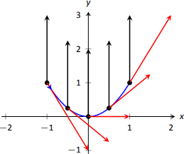
In Figure \(\PageIndex{2}\), we see the velocity and acceleration vectors for Object 1 plotted for \(t=-1, -1/2, 0, 1/2\) and \(t=1\). Note again how the constant acceleration vector seems to "pull'' the velocity vector from pointing down, right to up, right. We could plot the analogous picture for Object 2, but the velocity and acceleration vectors are rather large (\(\vecs a_2(-1) = \langle -6,30\rangle\)!)

Instead, we simply plot the locations of Object 1 and 2 on intervals of \(1/10^{\text{th}}\) of a second, shown in Figure \(\PageIndex{3a}\) and \(\PageIndex{3b}\)​​​​​​​ . Note how the \(x\)-values of Object 1 increase at a steady rate. This is because the \(x\)-component of \(\vecs a(t)\) is 0; there is no acceleration in the \(x\)-component. The dots are not evenly spaced; the object is moving faster near \(t=-1\) and \(t=1\) than near \(t=0\).

Figure \(\PageIndex{3}\)​​​​​​​: Comparing the positions of Objects 1 and 2 in Example 11.3.2

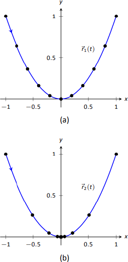
In Figure \(\PageIndex{3b}\)​​​​​​​, we see the points plotted for Object 2. Note the large change in position from \(t=-1\) to \(t=-0.9\); the object starts moving very quickly. However, it slows considerably at it approaches the origin, and comes to a complete stop at \(t=0\). While it looks like there are 3 points near the origin, there are in reality 5 points there.

Since the objects begin and end at the same location, the have the same displacement. Since they begin and end at the same time, with the same displacement, they have they have the same average rate of change (i.e, they have the same average velocity). Since they follow the same path, they have the same distance traveled. Even though these three measurements are the same, the objects obviously travel the path in very different ways.

Example \(\PageIndex{3}\): Analyzing the motion of a whirling ball on a string

A young boy whirls a ball, attached to a string, above his head in a counter-clockwise circle. The ball follows a circular path and makes 2 revolutions per second. The string has length 2ft.

1. Find the position function \(\vecs r(t)\) that describes this situation.
2. Find the acceleration of the ball and derive a physical interpretation of it.
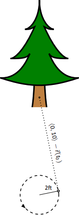
3. A tree stands 10 ft in front of the boy. At what \(t\)-values should the boy release the string so that the ball hits the tree?

Solution

1. The ball whirls in a circle. Since the string is 2 ft long, the radius of the circle is 2. The position function \(\vecs r (t)= \langle 2\cos t, 2\sin t\rangle\) describes a circle with radius 2, centered at the origin, but makes a full revolution every \(2\pi\) seconds, not two revolutions per second. We modify the period of the trigonometric functions to be 1/2 by multiplying \(t\) by \(4\pi\). The final position function is thus \[\vecs r (t) = \langle 2\cos (4\pi t), 2\sin (4\pi t)\rangle.\] (Plot this for \(0\leq t\leq 1/2\) to verify that one revolution is made in 1/2 a second.)
2. To find \(\vecs a (t)\), we derive \(\vecs r (t)\) twice. \[\begin{align*}\vecs v (t) = \vecs r^\prime (t) &= \langle -8\pi \sin (4\pi t), 8\pi \cos (4\pi t)\rangle\\[4pt] \vecs a (t) =\vecs r^{\prime\prime}(t) &= \langle -32\pi^2 \cos (4\pi t), -32\pi^2 \sin (4\pi t) \rangle \\[4pt]&= -32\pi^2\langle \cos (4\pi t), \sin (4\pi t)\rangle.\end{align*}\]
   
   Note how \(\vecs a (t)\) is parallel to \(\vecs r (t)\), but has a different magnitude and points in the opposite direction. Why is this?
   
   Recall the classic physics equation, "Force \(=\) mass \(\times\) acceleration.'' A force acting on a mass induces acceleration (i.e., the mass moves); acceleration acting on a mass induces a force (gravity gives our mass a weight). Thus force and acceleration are closely related. A moving ball "wants'' to travel in a straight line. Why does the ball in our example move in a circle? It is attached to the boy's hand by a string. The string applies a force to the ball, affecting it's motion: the string accelerates the ball. This is not acceleration in the sense of "it travels faster;'' rather, this acceleration is changing the velocity of the ball. In what direction is this force/acceleration being applied? In the direction of the string, towards the boy's hand.
   
   The magnitude of the acceleration is related to the speed at which the ball is traveling. A ball whirling quickly is rapidly changing direction/velocity. When velocity is changing rapidly, the acceleration must be "large.''
   
3. When the boy releases the string, the string no longer applies a force to the ball, meaning acceleration is \(\vecs 0\) and the ball can now move in a straight line in the direction of \(\vecs v(t)\).
   
   Let \(t=t_0\) be the time when the boy lets go of the string. The ball will be at \(\vecs r(t_0)\), traveling in the direction of \(\vecs v(t_0)\). We want to find \(t_0\) so that this line contains the point \((0,10)\) (since the tree is 10ft directly in front of the boy).
   
   There are many ways to find this time value. We choose one that is relatively simple computationally. As shown in Figure \(\PageIndex{4}\)​​​​​​​, the vector from the release point to the tree is \(\langle 0,10\rangle - \vecs r(t_0)\). This line segment is tangent to the circle, which means it is also perpendicular to \(\vecs r(t_0)\) itself, so their dot product is 0. \[ \begin{align*}\vecs r(t_0) \cdot \big(\langle 0,10\rangle - \vecs r(t_0)\big) &=0\\[4pt] \langle 2\cos (4\pi t_0), 2\sin (4\pi t_0)\rangle \cdot \langle -2\cos(4\pi t_0),10-2\sin (4\pi t_0)\rangle &=0\\[4pt]-4\cos^2(4\pi t_0) + 20\sin (4\pi t_0)-4\sin^2(4\pi t_0) &= 0\\[4pt]20\sin (4\pi t_0) - 4 &=0\\[4pt] \sin (4\pi t_0) &=1/5\\[4pt]4\pi t_0 &= \sin^{-1}(1/5)\\[4pt]4\pi t_0 &\approx 0.2 + 2\pi n, \end{align*}\] where \(n\) is an integer. Solving for \(t_0\) we have: \[t_0 \approx 0.016 + n/2\nonumber\] This is a wonderful formula. Every 1/2 second after \(t=0.016\)s the boy can release the string (since the ball makes 2 revolutions per second, he has two chances each second to release the ball).

Figure \(\PageIndex{4}\)​​​​​​​: Modeling the flight of a ball in Example 11.3.3

Example \(\PageIndex{4}\): Analyzing motion in space

An object moves in a spiral with position function \(\vecs r (t) = \langle \cos t, \sin t, t\rangle\), where distances are measured in meters and time is in minutes. Describe the object's speed and acceleration at time \(t\).

Solution
With \(\vecs r (t) = \langle \cos t,\sin t, t\rangle\), we have:

\[\begin{align*}
\vecs v (t) &= \langle -\sin t, \cos t, 1\rangle \quad \text{and} \\[4pt]
\vecs a (t) &= \langle -\cos t, -\sin t, 0\rangle.
\end{align*}\]

The speed of the object is \(\norm{\vecs v (t)} = \sqrt{(-\sin t)^2+\cos^2t+1} = \sqrt{2}\)m/min; it moves at a constant speed. Note that the object does not accelerate in the \(z\)-direction, but rather moves up at a constant rate of 1m/min.

The objects in Examples 11.3.3 and 11.3.4 traveled at a constant speed. That is, \(\norm{\vecs v (t)} = c\) for some constant \(c\). Recall Theorem 93, which states that if a vector--valued function \(\vecs r (t)\)\ has constant length, then \(\vecs r (t)\)\ is perpendicular to its derivative: \(\vecs r (t)\cdot\vecs r^\prime (t) = 0\). In these examples, the velocity function has constant length, therefore we can conclude that the velocity is perpendicular to the acceleration: \(\vecs v (t)cdot\vecs a (t) = 0\). A quick check verifies this.

There is an intuitive understanding of this. If acceleration is parallel to velocity, then it is only affecting the object's speed; it does not change the direction of travel. (For example, consider a dropped stone. Acceleration and velocity are parallel -- straight down -- and the direction of velocity never changes, though speed does increase.) If acceleration is not perpendicular to velocity, then there is some acceleration in the direction of travel, influencing the speed. If speed is constant, then acceleration must be orthogonal to velocity, as it then only affects direction, and not speed.

key idea: 52 Objects With Constant Speed

If an object moves with constant speed, then its velocity and acceleration vectors are orthogonal. That is, \(\vecs v (t)cdot\vecs a (t)=0\).

Projectile Motion

An important application of vector--valued position functions is projectile motion: the motion of objects under only the influence of gravity. We will measure time in seconds, and distances will either be in meters or feet. We will show that we can completely describe the path of such an object knowing its initial position and initial velocity (i.e., where it is and where it is going.)

Suppose an object has initial position \(\vecs r(0) = \langle x_0,y_0\rangle\) and initial velocity \(\vecs v(0) = \langle v_x,v_y\rangle\). It is customary to rewrite \(\vecs v(0)\) in terms of its speed \(v_0\) and direction \(\vecs u\), where \(\vecs u\) is a unit vector. Recall all unit vectors in \(\mathbb{R}^2\) can be written as \(\langle \cos \theta,\sin \theta\rangle\), where \(\theta\) is an angle measure counter--clockwise from the \(x\)-axis. (We refer to \(\theta\) as the angle of elevation.) Thus \(\vecs v(0) = v_0\langle \cos \theta,\sin \theta\rangle.\)

Since the acceleration of the object is known, namely \(\vecs a (t) = \langle 0,-g\rangle\), where \(g\) is the gravitational constant, we can find \(\vecs r (t)\) knowing our two initial conditions. We first find \(\vecs v (t)):

Note

In this text we use \(g=32\)ft/s when using Imperial units, and \(g=9.8\)m/s when using SI units.

\[\begin{align*}
\vecs v(t) &= \int \vecs a (t) dt \\[4pt]
\vecs v (t) &= \int \langle 0,-g\rangle dt \\[4pt]
\vecs v (t) &= \langle 0,-gt\rangle + \vecs C.
\end{align*}\]

Knowing \(\vecs v(0) = v_0\langle \cos \theta,\sin \theta\rangle\), we have \(\vecs C = v_0\langle \cos t,\sin t\rangle\) and so

\[\vecs v(t) = \langle v_0\cos \theta, -gt+v_0\sin\theta\rangle.\]

We integrate once more to find \(\vecs r (t)\):

\[\begin{align*}
\vecs r (t) &= \int \vecs v (t) dt \\[4pt]
\vecs r (t) &= \int \langle v_0\cos \theta, -gt+v_0\sin\theta\rangle dt \\[4pt]
\vecs r (t) &= \langle \big(v_0\cos \theta\big)t, -\dfrac12gt^2+\big(v_0\sin\theta\big)t\rangle + \vecs C. \\[4pt]
\text{Knowing \(\vecs r(0) = \langle x_0,y_0\rangle\), we conclude \(\vecs C = \langle x_0,y_0\rangle\) and }& \\[4pt]
\vecs r (t) &= \langle \big(v_0\cos \theta\big)t+x_0\ , -\dfrac12gt^2+\big(v_0\sin\theta\big)t+y_0\ \rangle.
\end{align*}\]

key idea 53: Projectile Motion

The position function of a projectile propelled from an initial position of \(\vecs r_0=\langle x_0,y_0\rangle\), with initial speed \(v_0\), with angle of elevation \(\theta\) and neglecting all accelerations but gravity is

\[\vecs r (t) = \langle \big(v_0\cos \theta\big)t+x_0\ , -\dfrac12gt^2+\big(v_0\sin\theta\big)t+y_0\ \rangle.\]

Letting \(\vecs v_0 = v_0\langle \cos \theta,\sin \theta\rangle\), (\vecs r (t)\) can be written as

\[\vecs r (t) = \langle 0,-\dfrac12gt^2\rangle + \vecs v_0t+\vecs r_0.\]

We demonstrate how to use this position function in the next two examples.

Example \(\PageIndex{5}\): Projectile Motion

Sydney shoots her Red Ryder bb gun across level ground from an elevation of 4ft, where the barrel of the gun makes a \(5^\circ\) angle with the horizontal. Find how far the bb travels before landing, assuming the bb is fired at the advertised rate of 350ft/s and ignoring air resistance.

Solution

A direct application of Key Idea 53 gives

\[\begin{align*}
\vecs r (t) &= \langle (350\cos 5^\circ)t, -16t^2 + (350\sin 5^\circ)t + 4\rangle\\[4pt]
&\approx \langle 346.67t, -16t^2+30.50t+4\rangle,
\end{align*}\]

where we set her initial position to be \(\langle 0,4\rangle\).
We need to find when the bb lands, then we can find where. We accomplish this by setting the \(y\)-component equal to 0 and solving for \(t\):

\[\begin{align*}
-16t^2+30.50t+4 &= 0 \\[4pt]
t &= \dfrac{-30.50 \pm \sqrt{30.50^2-4(-16)(4)}}{-32}\\[4pt]
t &\approx 2.03s.
\end{align*}\]

(We discarded a negative solution that resulted from our quadratic equation.)

We have found that the bb lands 2.03s after firing; with \(t=2.03\), we find the \(x\)-component of our position function is \(346.67(2.03) = 703.74\)ft. The bb lands about 704 feet away.

Example \(\PageIndex{6}\): Projectile Motion

Alex holds his sister's bb gun at a height of 3ft and wants to shoot a target that is 6ft above the ground, 25ft away. At what angle should he hold the gun to hit his target? (We still assume the muzzle velocity is 350ft/s.)

Solution

The position function for the path of Alex's bb is

\[\vecs r (t) = \langle (350\cos \theta)t, -16t^2+(350\sin\theta)t+3\rangle. \nonumber\]

We need to find \(\theta\) so that \(\vecs r (t)\) =\langle 25,6\rangle\) for some value of \(t\). That is, we want to find \(\theta\) and \(t\) such that

\[(350\cos\theta)t = 25 \quad \text{and}\quad -16t^2+(350\sin\theta)t+3 = 6. \nonumber\]

This is not trivial (though not "hard''). We start by solving each equation for \(\cos\theta\) and \(\sin \theta\), respectively.

\[\cos\theta = \dfrac{25}{350t} \quad \text{and} \quad \sin\theta = \dfrac{3+16t^2}{350t}. \nonumber\]

Using the Pythagorean Identity \(\cos^2\theta+\sin^2\theta=1\), we have

\[\left(\dfrac{25}{350t}\right)^2 + \left(\dfrac{3+16t^2}{350t}\right)^2 =1 \nonumber\]

Multiply both sides by \((350t)^2\):

\[\begin{align*}25^2 + (3+16t^2)^2 &=350^2t^2\\[4pt] 256t^4-122,404t^2+634 &=0.\end{align*}\]

This is a quadratic in \(t^2\). That is, we can apply the quadratic formula to find \(t^2\), then solve for \(t\) itself.

\[\begin{align*}
t^2 &= \dfrac{122,404\pm\sqrt{122,404^2-4(256)(634)}}{512}\\[4pt]
t^2 &= 0.0052,\ 478.135\\[4pt]
t &= \pm 0.072,\ \pm 21.866
\end{align*}\]

Clearly the negative \(t\) values do not fit our context, so we have \(t=0.072\) and \(t=21.866\). Using \(\cos \theta = 25/(350 t)\), we can solve for \(\theta\):

\[\begin{align*}
\theta &= \cos^{-1}\left(\dfrac{25}{350\cdot 0.072}\right)\quad \text{and}\quad \cos^{-1}\left(\dfrac{25}{350\cdot 21.866}\right)\\[4pt]
\theta &= 7.03^\circ \quad \text{and} \quad 89.8^\circ.
\end{align*}\]

Alex has two choices of angle. He can hold the rifle at an angle of about \(7^\circ\) with the horizontal and hit his target \(0.07\)s after firing, or he can hold his rifle almost straight up, with an angle of \(89.8^\circ\), where he'll hit his target about 22s later. The first option is clearly the option he should choose.

Distance Traveled

Consider a driver who sets her cruise--control to 60mph, and travels at this speed for an hour. We can ask:

1. How far did the driver travel?
2. How far from her starting position is the driver?

The first is easy to answer: she traveled 60 miles. The second is impossible to answer with the given information. We do not know if she traveled in a straight line, on an oval racetrack, or along a slowly--winding highway.

This highlights an important fact: to compute distance traveled, we need only to know the speed, given by \(\norm{\vecs v (t)}\).

theorem 96: Distance Traveled

Let \(\vecs v (t)\) be a velocity function for a moving object. The distance traveled by the object on \([a,b]\) is:

\[\text{distance traveled} = \int_a^b \norm{\vecs v (t)} dt .\]

Note that this is just a restatement of Theorem 95: arc length is the same as distance traveled, just viewed in a different context.

Example \(\PageIndex{7}\): Distance Traveled, Displacement, and Average Speed

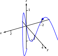
A particle moves in space with position function \(\vecs r (t) = \langle t,t^2,\sin (\pi t)\rangle\) on \([-2,2]\), where \(t\) is measured in seconds and distances are in meters. Find:

1. The distance traveled by the particle on \([-2,2]\).
2. The displacement of the particle on \([-2,2]\).
3. The particle's average speed.

Solution

1. We use Theorem 96 to establish the integral: \[\begin{align*}\text{distance traveled} &= \int_{-2}^2 \norm{\vecs v (t)} dt \\[4pt]&= \int_{-2}^2 \sqrt{1+(2t)^2+ \pi^2\cos^2(\pi t)} dt .\end{align*}\] This cannot be solved in terms of elementary functions so we turn to numerical integration, finding the distance to be 12.88m.
2. The displacement is the vector \[\vecs r(2)-\vecs r(-2) = \langle 2,4,0\rangle - \langle -2,4,0\rangle = \langle 4,0,0\rangle. \nonumber\] That is, the particle ends with an \(x\)-value increased by 4 and with \(y\)- and \(z\)-values the same (see Figure \(\PageIndex{5}\)​​​​​​​).
3. We found above that the particle traveled 12.88m over 4 seconds. We can compute average speed by dividing: 12.88/4 = 3.22m/s.
   
   We should also consider Definition 22 of Section 5.4, which says that the average value of a function \(f\) on \([a,b]\) is \(\dfrac{1}{b-a}\int_a^b f(x)\ dx\). In our context, the average value of the speed is \[\text{average speed} = \dfrac{1}{2-(-2)}\int_{-2}^2 \norm{\vecs v (t)} dt \approx \dfrac14 12.88 = 3.22\text{m/s}. \nonumber \]
   
   Note how the physical context of a particle traveling gives meaning to a more abstract concept learned earlier.

Figure \(\PageIndex{5}\)​​​​​​​: The path of the particle in Example 11.3.7

In Definition 22 of Chapter 5 we defined the average value of a function \(f(x)\) on \([a,b]\) to be

\[ \dfrac{1}{b-a}\int_a^bf(x) dx.\]

Note how in Example 11.3.7 we computed the average speed as

\[\dfrac{\text{distance traveled}}{\text{travel time}} = \dfrac1{2-(-2)}\int_{-2}^2\norm{\vecs v (t)} dt ;\]

that is, we just found the average value of \(\norm{\vecs v (t)}\) on \([-2,2]\).

Likewise, given position function \(\vecs r (t)\), the average velocity on \([a,b]\) is

\[\dfrac{\text{displacement}}{\text{travel time}} = \dfrac1{b-a}\int_a^b \vecs{r}\,'(t) dt = \dfrac{\vecs r(b)-\vecs r(a)}{b-a};\]

that is, it is the average value of \(\vecs r\,'(t)\), or \(\vecs v (t)\), on \([a,b]\).

KEY IDEA 54: Average Speed, Average Velocity

Let \(\vecs r(t)\) be a continuous position function on an open interval \(I\) containing \(a<b\).

• The average speed is:

\[\dfrac{\text{distance traveled}}{\text{travel time}} = \dfrac{\int_a^b \norm{\vecs v (t)} dt }{b-a} = \dfrac1{b-a}\int_a^b\norm{\vecs v (t)} dt .\]

• The average velocity is:

\[\dfrac{\text{displacement}}{\text{travel time}} = \dfrac{\int_a^b \vecs{r}\,'(t) dt }{b-a} = \dfrac1{b-a}\int_a^b\vecs{r}\,'(t) dt .\]

The next two sections investigate more properties of the graphs of vector--valued functions and we'll apply these new ideas to what we just learned about motion.