12.8: Extreme Values

Given a function \(z=f(x,y)\), we are often interested in points where \(z\) takes on the largest or smallest values. For instance, if \(z\) represents a cost function, we would likely want to know what \((x,y)\) values minimize the cost. If \(z\) represents the ratio of a volume to surface area, we would likely want to know where \(z\) is greatest. This leads to the following definition.

Definition 97 Relative and Absolute Extrema

Let \(z=f(x,y)\) be defined on a set \(S\) containing the point \(P=(x_0,y_0)\).

1. If there is an open disk \(D\) containing \(P\) such that \(f(x_0,y_0) \geq f(x,y)\) for all \((x,y)\) in \(D\), then \(f\) has a relative maximum at \(P\); if \(f(x_0,y_0) \leq f(x,y)\) for all \((x,y)\) in \(D\), then \(f\) has a relative minimum at \(P\).
2. If \(f(x_0,y_0)\geq f(x,y)\) for all \((x,y)\) in \(S\), then \(f\) has an absolute maximum at \(P\); if \(f(x_0,y_0)\leq f(x,y)\) for all \((x,y)\) in \(S\), then \(f\) has an absolute minimum at \(P\).
3. If \(f\) has a relative maximum or minimum at \(P\), then \(f\) has a relative extrema at \(P\); if \(f\) has an absolute maximum or minimum at \(P\), then \(f\) has an absolute extrema at \(P\).

If \(f\) has a relative or absolute maximum at \(P=(x_0,y_0)\), it means every curve on the surface of \(f\) through \(P\) will also have a relative or absolute maximum at \(P\). Recalling what we learned in Section 3.1, the slopes of the tangent lines to these curves at \(P\) must be 0 or undefined. Since directional derivatives are computed using \(f_x\) and \(f_y\), we are led to the following definition and theorem.

Definition 98 Critical Point

Let \(z = f(x,y)\) be continuous on an open set \(S\). A critical point \(P=(x_0,y_0)\) of \(f\) is a point in \(S\) such that

• \(f_x(x_0,y_0) = 0\) and \(f_y(x_0,y_0) = 0\), or
• \(f_x(x_0,y_0)\) and/or \(f_y(x_0,y_0)\) is undefined.

theorem 114 Critical Points and Relative Extrema

Let \(z=f(x,y)\) be defined on an open set \(S\) containing \(P=(x_0,y_0)\). If \(f\) has a relative extrema at \(P\), then \(P\) is a critical point of \(f\).

Therefore, to find relative extrema, we find the critical points of \(f\) and determine which correspond to relative maxima, relative minima, or neither. The following examples demonstrate this process.

Example \(\PageIndex{1}\): Finding critical points and relative extrema

Let \(f(x,y) = x^2+y^2-xy-x-2\). Find the relative extrema of \(f\).

Solution

We start by computing the partial derivatives of \(f\):

\[f_x(x,y) = 2x-y-1 \qquad \text{and}\qquad f_y(x,y) = 2y-x.\]

Each is never undefined. A critical point occurs when \(f_x\) and \(f_y\) are simultaneously 0, leading us to solve the following system of linear equations:

\[2x-y-1 = 0\qquad \text{and}\qquad -x+2y = 0.\]

This solution to this system is \(x=2/3\), \(y=1/3\). (Check that at \((2/3,1/3)\), both \(f_x\) and \(f_y\) are 0.)

Figure 12.27: The surface in Example 12.8.1 with its absolute minimum indicated.

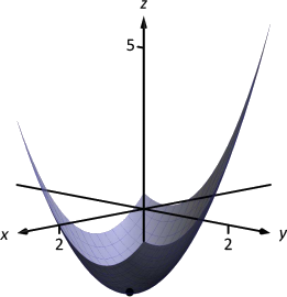
The graph in Figure 12.27 shows \(f\) along with this critical point. It is clear from the graph that this is a relative minimum; further consideration of the function shows that this is actually the absolute minimum.

Example \(\PageIndex{2}\): Finding critical points and relative extrema

Let \(f(x,y) = -\sqrt{x^2+y^2}+2\). Find the relative extrema of \(f\).

Solution

We start by computing the partial derivatives of \(f\):

\[f_x(x,y) = \frac{-x}{\sqrt{x^2+y^2}}\qquad \text{and}\qquad f_y(x,y) = \frac{-y}{\sqrt{x^2+y^2}}.\]

It is clear that \(f_x=0\) when \(x=0\) \& \(y\neq0\), and that \(f_y=0\) when \(y=0\) \& \(x\neq0\). At \((0,0)\), both \(f_x\) and \(f_y\) are not \(0\), but rather undefined. The point \((0,0)\) is still a critical point, though, because the partial derivatives are undefined. This is the only critical point of \(f\).

Figure 12.28: The surface in Example 12.8.2 with its absolute maximum indicated.

The surface of \(f\) is graphed in Figure 12.28 along with the point \((0,0,2)\). The graph shows that this point is the absolute maximum of \(f\).

In each of the previous two examples, we found a critical point of \(f\) and then determined whether or not it was a relative (or absolute) maximum or minimum by graphing. It would be nice to be able to determine whether a critical point corresponded to a max or a min without a graph. Before we develop such a test, we do one more example that sheds more light on the issues our test needs to consider.

Example \(\PageIndex{3}\): Finding critical points and relative extrema

Let \(f(x,y) = x^3-3x-y^2+4y\). Find the relative extrema of \(f\).

Solution

Once again we start by finding the partial derivatives of \(f\):

\[f_x(x,y) = 3x^2-3\qquad \text{and} \qquad f_y(x,y) = -2y+4.\]

Each is always defined. Setting each equal to 0 and solving for \(x\) and \(y\), we find

\[\begin{align*}
f_x(x,y) = 0 \quad &\Rightarrow x=\pm 1\\
f_y(x,y) = 0\quad &\Rightarrow y = 2.
\end{align*}\]

We have two critical points: \((-1,2)\) and \((1,2)\). To determine if they correspond to a relative maximum or minimum, we consider the graph of \(f\) in Figure 12.29.

Figure 12.29: The surface in Example 12.8.3 with both critical points marked.

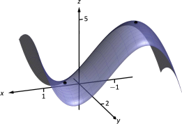
The critical point \((-1,2)\) clearly corresponds to a relative maximum. However, the critical point at \((1,2)\) is neither a maximum nor a minimum, displaying a different, interesting characteristic.

If one walks parallel to the \(y\)-axis towards this critical point, then this point becomes a relative maximum along this path. But if one walks towards this point parallel to the \(x\)-axis, this point becomes a relative minimum along this path. A point that seems to act as both a max and a min is a saddle point. A formal definition follows.

Definition 99 Saddle Point

Let \(P=(x_0,y_0)\) be in the domain of \(f\) where \(f_x=0\) and \(f_y=0\) at \(P\). \(P\) is a saddle point of \(f\) if, for every open disk \(D\) containing \(P\), there are points \((x_1,y_1)\) and \((x_2,y_2)\) in \(D\) such that \(f(x_0,y_0)>f(x_1,y_1)\) and \(f(x_0,y_0)<f(x_2,y_2)\).

At a saddle point, the instantaneous rate of change in all directions is 0 and there are points nearby with \(z\)-values both less than and greater than the \(z\)-value of the saddle point.

Before Example 12.8.3 we mentioned the need for a test to differentiate between relative maxima and minima. We now recognize that our test also needs to account for saddle points. To do so, we consider the second partial derivatives of \(f\).

Recall that with single variable functions, such as \(y=f(x)\), if \(f''(c)>0\), then \(f\) is concave up at \(c\), and if \(f'(c) =0\), then \(f\) has a relative minimum at \(x=c\). (We called this the Second Derivative Test.) Note that at a saddle point, it seems the graph is "both'' concave up and concave down, depending on which direction you are considering.

It would be nice if the following were true:

However, this is not the case. Functions \(f\) exist where \(f_{xx}\) and \(f_{yy}\) are both positive but a saddle point still exists. In such a case, while the concavity in the \(x\)-direction is up (i.e., \(f_{xx}>0\)) and the concavity in the \(y\)-direction is also up (i.e., \(f_{yy}>0\)), the concavity switches somewhere in between the \(x\)- and \(y\)-directions.

To account for this, consider \(D = f_{xx}f_{yy}-f_{xy}f_{yx}\). Since \(f_{xy}\) and \(f_{yx}\) are equal when continuous (refer back to Theorem 103), we can rewrite this as \(D = f_{xx}f_{yy}-f_{xy}^{\,2}\). \(D\) can be used to test whether the concavity at a point changes depending on direction. If \(D>0\), the concavity does not switch (i.e., at that point, the graph is concave up or down in all directions). If \(D<0\), the concavity does switch. If \(D=0\), our test fails to determine whether concavity switches or not. We state the use of \(D\) in the following theorem.

THEOREM 115 Second Derivative Test

Let \(z=f(x,y)\) be differentiable on an open set containing \(P = (x_0,y_0)\), and let
\[D = f_{xx}(x_0,y_0)f_{yy}(x_0,y_0)-f_{xy}^{\,2}(x_0,y_0).\]

1. If \(D>0\) and \(f_{xx}(x_0,y_0)>0\), then \(P\) is a relative minimum of \(f\).
2. If \(D>0\) and \(f_{xx}(x_0,y_0)<0\), then \(P\) is a relative maximum of \(f\).
3. If \(D<0\), then \(P\) is a saddle point of \(f\).
4. If \(D=0\), the test is inconclusive.

We first practice using this test with the function in the previous example, where we visually determined we had a relative maximum and a saddle point.

Example \(\PageIndex{4}\): Using the Second Derivative Test

Let \(f(x,y) = x^3-3x-y^2+4y\) as in Example 12.8.3. Determine whether the function has a relative minimum, maximum, or saddle point at each critical point.

Solution
We determined previously that the critical points of \(f\) are \((-1,2)\) and \((1,2)\). To use the Second Derivative Test, we must find the second partial derivatives of \(f\):
\[f_{xx} = 6x;\qquad f_{yy} = -2;\qquad f_{xy} = 0.\]
Thus \(D(x,y) = -12x\).

At \((-1,2)\): \(D(-1,2) = 12>0\), and \(f_{xx}(-1,2) = -6\). By the Second Derivative Test, \(f\) has a relative maximum at \((-1,2)\).

At \((1,2)\): \(D(1,2) = -12 <0\). The Second Derivative Test states that \(f\) has a saddle point at \((1,2)\).

The Second Derivative Test confirmed what we determined visually.

Example \(\PageIndex{5}\): Using the Second Derivative Test

Find the relative extrema of \(f(x,y) = x^2y+y^2+xy\).

Solution

We start by finding the first and second partial derivatives of \(f\):

\[\begin{array}{ccc}
f_x = 2xy+y & & f_y = x^2+2y+x \\
f_{xx} = 2y & & f_{yy} = 2\\
f_{xy} = 2x+1 & & f_{yx} = 2x+1.
\end{array}\]

We find the critical points by finding where \(f_x\) and \(f_y\) are simultaneously 0 (they are both never undefined). Setting \(f_x=0\), we have:

\[f_x=0 \quad \Rightarrow \quad 2xy+y=0\quad \Rightarrow \quad y(2x+1)=0.\]

This implies that for \(f_x=0\), either \(y=0\) or \(2x+1=0\).

Assume \(y=0\) then consider \(f_y=0\):

\[\begin{align*}
f_y &= 0\\
x^2+2y+x &= 0, \qquad \text{and since \(y=0\), we have}\\
x^2+x &= 0\\
x(x+1) & = 0.
\end{align*}\]

Thus if \(y=0\), we have either \(x=0\) or \(x=-1\), giving two critical points: \((-1,0)\) and \((0,0)\).

Going back to \(f_x\), now assume \(2x+1=0\), i.e., that \(x=-1/2\), then consider \(f_y=0\):

\[\begin{align*}
f_y &= 0\\
x^2+2y+x &= 0, \qquad \text{and since \(x=-1/2\), we have}\\
1/4+2y-1/2 &= 0\\
y&= 1/8.
\end{align*}\]

Thus if \(x=-1/2\), \(y=1/8\) giving the critical point \((-1/2,1/8)\).

With \(D = 4y-(2x+1)^2\), we apply the Second Derivative Test to each critical point.

At \((-1,0)\), \(D <0\), so \((-1,0)\) is a saddle point.

At \((0,0)\), \(D<0\), so \((0,0)\) is also a saddle point.

At \((-1/2,1/8)\), \(D>0\) and \(f_{xx} > 0\), so \((-1/2,1/8)\) is a relative minimum.

Figure 12.30: Graphing \(f\) from Example 12.8.5 and its relative extrema.

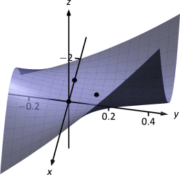
Figure 12.30 shows a graph of \(f\) and the three critical points. Note how this function does not vary much near the critical points -- that is, visually it is difficult to determine whether a point is a saddle point or relative minimum (or even a critical point at all!). This is one reason why the Second Derivative Test is so important to have.

Constrained Optimization

When optimizing functions of one variable such as \(y=f(x)\), we made use of Theorem 25, the Extreme Value Theorem, that said that over a closed interval \(I\), a continuous function has both a maximum and minimum value. To find these maximum and minimum values, we evaluated \(f\) at all critical points in the interval, as well as at the endpoints (the "boundary'') of the interval.

A similar theorem and procedure applies to functions of two variables. A continuous function over a closed set also attains a maximum and minimum value (see the following theorem). We can find these values by evaluating the function at the critical values in the set and over the boundary of the set. After formally stating this extreme value theorem, we give examples.

theorem 116 Extreme Value Theorem

Let \(z=f(x,y)\) be a continuous function on a closed, bounded set \(S\). Then \(f\) has a maximum and minimum value on \(S\).

Example \(\PageIndex{6}\): Finding extrema on a closed set

Let \(f(x,y) = x^2-y^2+5\) and let \(S\) be the triangle with vertices \((-1,-2)\), \((0,1)\) and \((2,-2)\). Find the maximum and minimum values of \(f\) on \(S\).

Solution
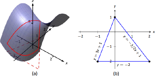
It can help to see a graph of \(f\) along with the set \(S\). In Figure 12.31(a) the triangle defining \(S\) is shown in the \(xy\)-plane in a dashed line. Above it is the surface of \(f\); we are only concerned with the portion of \(f\) enclosed by the "triangle'' on its surface.

Figure 12.31: Plotting the surface of \(f\) along with the restricted domain S.

We begin by finding the critical points of \(f\). With \(f_x = 2x\) and \(f_y = -2y\), we find only one critical point, at \((0,0)\).

We now find the maximum and minimum values that \(f\) attains along the boundary of \(S\), that is, along the edges of the triangle. In Figure 12.31(b) we see the triangle sketched in the plane with the equations of the lines forming its edges labeled.

Start with the bottom edge, along the line \(y=-2\). If \(y\) is \(-2\), then on the surface, we are considering points \(f(x,-2)\); that is, our function reduces to \(f(x,-2) = x^2-(-2)^2+5 = x^2+1=f_1(x)\). We want to maximize/minimize \(f_1(x)=x^2+1\) on the interval \([-1,2]\). To do so, we evaluate \(f_1(x)\) at its critical points and at the endpoints.

The critical points of \(f_1\) are found by setting its derivative equal to 0:
\[f'_1(x)=0\qquad \Rightarrow x=0.\]
Evaluating \(f_1\) at this critical point, and at the endpoints of \([-1,2]\) gives:
\[\begin{align*}
f_1(-1) = 2 \qquad&\Rightarrow\qquad f(-1,-2) = 2\\
f_1(0) = 1 \qquad&\Rightarrow \qquad f(0,-2) = 1\\
f_1(2) = 5 \qquad&\Rightarrow \qquad f(2,-2) = 5.
\end{align*}\]
Notice how evaluating \(f_1\) at a point is the same as evaluating \(f\) at its corresponding point.

We need to do this process twice more, for the other two edges of the triangle.

Along the left edge, along the line \(y=3x+1\), we substitute \(3x+1\) in for \(y\) in \(f(x,y)\):
\[f(x,y) = f(x,3x+1) = x^2-(3x+1)^2+5 = -8x^2-6x+4 = f_2(x).\]
We want the maximum and minimum values of \(f_2\) on the interval \([-1,0]\), so we evaluate \(f_2\) at its critical points and the endpoints of the interval. We find the critical points:
\[f'_2(x) = -16x-6=0 \qquad \Rightarrow \qquad x=-3/8.\]

Evaluate \(f_2\) at its critical point and the endpoints of \([-1,0]\):
\[\begin{align*}
f_2(-1) = 2 \qquad&\Rightarrow\qquad f(-1,-2) = 2\\
f_2(-3/8) = 41/8=5.125 \qquad&\Rightarrow \qquad f(-3/8,-0.125) = 5.125\\
f_2(0) = 1 \qquad&\Rightarrow \qquad f(0,1) = 4.
\end{align*}\]

Finally, we evaluate \(f\) along the right edge of the triangle, where \(y = -3/2x+1\).
\[f(x,y) = f(x,-3/2x+1) = x^2-(-3/2x+1)^2+5 = -\frac54x^2+3x+4=f_3(x).\]
The critical points of \(f_3(x)\) are:
\[f'_3(x) = 0 \qquad \Rightarrow \qquad x=6/5=1.2.\]
We evaluate \(f_3\) at this critical point and at the endpoints of the interval \([0,2]\):
\[\begin{align*}
f_3(0) = 4 \qquad&\Rightarrow\qquad f(0,1) = 4\\
f_3(1.2) = 5.8 \qquad&\Rightarrow \qquad f(1.2,-0.8) = 5.8\\
f_3(2) = 5 \qquad&\Rightarrow \qquad f(2,-2) = 5.
\end{align*}\]
One last point to test: the critical point of \(f\), \((0,0)\). We find \(f(0,0) = 5\).

Figure 12.32: The surface of \(f\) along with important points along the boundary of S and the interior.

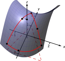
We have evaluated \(f\) at a total of 7 different places, all shown in Figure 12.32. We checked each vertex of the triangle twice, as each showed up as the endpoint of an interval twice. Of all the \(z\)-values found, the maximum is 5.8, found at \((1.2,-0.8)\); the minimum is 1, found at \((0,-2)\).

This portion of the text is entitled "Constrained Optimization'' because we want to optimize a function (i.e., find its maximum and/or minimum values) subject to a constraint -- limits on which input points are considered. In the previous example, we constrained ourselves by considering a function only within the boundary of a triangle. This was largely arbitrary; the function and the boundary were chosen just as an example, with no real "meaning'' behind the function or the chosen constraint.

However, solving constrained optimization problems is a very important topic in applied mathematics. The techniques developed here are the basis for solving larger problems, where more than two variables are involved.

We illustrate the technique once more with a classic problem.

Example \(\PageIndex{7}\): Constrained Optimization

The U.S. Postal Service states that the girth+length of Standard Post Package must not exceed 130''. Given a rectangular box, the "length'' is the longest side, and the "girth'' is twice the width+height.

Given a rectangular box where the width and height are equal, what are the dimensions of the box that give the maximum volume subject to the constraint of the size of a Standard Post Package?

Solution

Let \(w\), \(h\) and \(\ell\) denote the width, height and length of a rectangular box; we assume here that \(w=h\). The girth is then \(2(w+h) = 4w\). The volume of the box is \(V(w,\ell) = wh\ell = w^2\ell\). We wish to maximize this volume subject to the constraint \(4w+\ell\leq 130\), or \(\ell\leq 130-4w\). (Common sense also indicates that \(\ell>0, w>0\).)

We begin by finding the critical values of \(V\). We find that \(V_w = 2w\ell\) and \(V_\ell = w^2\); these are simultaneously 0 only at \((0,0)\). This gives a volume of 0, so we can ignore this critical point.

We now consider the volume along the constraint \(\ell=130-4w.\) Along this line, we have:
\[V(w,\ell) = V(w,130-4w) = w^2(130-4w) = 130w^2-4w^3 = V_1(w).\]
The constraint is applicable on the \(w\)-interval \([0,32.5]\) as indicated in the figure. Thus we want to maximize \(V_1\) on \([0,32.5]\).

Finding the critical values of \(V_1\), we take the derivative and set it equal to 0:
\[V\,'_1(w) = 260w-12w^2 = 0 \quad \Rightarrow \quad w(260-12w)= 0 \quad \Rightarrow \quad w=0,\frac{260}{12}\approx 21.67.\]

We found two critical values: when \(w=0\) and when \(w=21.67\). We again ignore the \(w=0\) solution; the maximum volume, subject to the constraint, comes at \(w=h=21.67\), \(\ell = 130-4(21.6) =43.33.\) This gives a volume of \(V(21.67,43.33) \approx 19,408\)in\(^3\).

Figure 12.33: Graphing the volume of a box with girth 4w and length \(l\), subject to a size constraint.

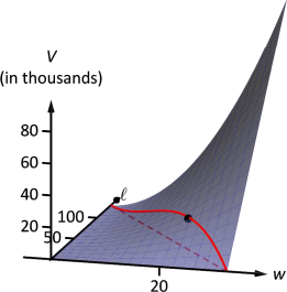
The volume function \(V(w,\ell)\) is shown in Figure 12.33 along with the constraint \(\ell = 130-4w\). As done previously, the constraint is drawn dashed in the \(xy\)-plane and also along the surface of the function. The point where the volume is maximized is indicated.

It is hard to overemphasize the importance of optimization. In "the real world,'' we routinely seek to make something better. By expressing the something as a mathematical function, "making something better'' means "optimize some function.''

The techniques shown here are only the beginning of an incredibly important field. Many functions that we seek to optimize are incredibly complex, making the step of "find the gradient and set it equal to \(\vec 0\)'' highly nontrivial. Mastery of the principles here is key to being able to tackle these more complicated problems.

Contributors and Attributions

• Gregory Hartman (Virginia Military Institute). Contributions were made by Troy Siemers and Dimplekumar Chalishajar of VMI and Brian Heinold of Mount Saint Mary's University. This content is copyrighted by a Creative Commons Attribution - Noncommercial (BY-NC) License. http://www.apexcalculus.com/