13.1: Iterated Integrals and Area

In the previous chapter we found that we could differentiate functions of several variables with respect to one variable, while treating all the other variables as constants or coefficients. We can integrate functions of several variables in a similar way. For instance, if we are told that $f_x(x,y) = 2xy$, we can treat $y$ as staying constant and integrate to obtain $f(x,y)$:

$$\begin{align*} f(x,y) &= \int f_x(x,y) \,dx\\ &= \int 2xy \,dx \\ &= x^2y + C. \end{align*}$$

Make a careful note about the constant of integration, $C$. This "constant'' is something with a derivative of $0$ with respect to $x$, so it could be any expression that contains only constants and functions of $y$. For instance, if $f(x,y) = x^2y+ \sin y + y^3 + 17$, then $f_x(x,y) = 2xy$. To signify that $C$ is actually a function of $y$, we write:

$$f(x,y) = \int f_x(x,y) \,dx = x^2y+C(y).$$

Using this process we can even evaluate definite integrals.

Example $\PageIndex{1}$: Integrating functions of more than one variable

Evaluate the integral $\displaystyle \int_1^{2y} 2xy \,dx.$

Solution

We find the indefinite integral as before, then apply the Fundamental Theorem of Calculus to evaluate the definite integral:

$$\begin{align*} \int_1^{2y} 2xy \,dx &= x^2y\Big|_1^{2y}\\ &= (2y)^2y - (1)^2y \\ &= 4y^3-y. \end{align*}$$

We can also integrate with respect to $y$. In general,

$$\int_{h_1(y)}^{h_2(y)} f_x(x,y) \,dx = f(x,y)\Big|_{h_1(y)}^{h_2(y)} = f\big(h_2(y),y\big)-f\big(h_1(y),y\big),$$

and

$$\int_{g_1(x)}^{g_2(x)} f_y(x,y) \,dy = f(x,y)\Big|_{g_1(x)}^{g_2(x)} = f\big(x,g_2(x)\big)-f\big(x,g_1(x)\big).$$

Note that when integrating with respect to $x$, the bounds are functions of $y$ (of the form $x=h_1(y)$ and $x=h_2(y)$) and the final result is also a function of $y$. When integrating with respect to $y$, the bounds are functions of $x$ (of the form $y=g_1(x)$ and $y=g_2(x)$) and the final result is a function of $x$. Another example will help us understand this.

Example $\PageIndex{2}$: Integrating functions of more than one variable

Evaluate $\displaystyle \int_1^x\big(5x^3y^{-3}+6y^2\big) \,dy$.

Solution

We consider $x$ as staying constant and integrate with respect to $y$:

$$\begin{align*} \int_1^x\big(5x^3y^{-3}+6y^2\big) \,dy & = \left(\frac{5x^3y^{-2}}{-2}+\frac{6y^3}{3}\right)\Bigg|_1^x \\ &= \left(-\frac52x^3x^{-2}+2x^3\right) - \left(-\frac52x^3+2\right) \\ &= \frac92x^3-\frac52x-2. \end{align*}$$

Note how the bounds of the integral are from $y=1$ to $y=x$ and that the final answer is a function of $x$.

In the previous example, we integrated a function with respect to $y$ and ended up with a function of $x$. We can integrate this as well. This process is known as iterated integration, or multiple integration.

Example $\PageIndex{3}$: Integrating an integral

Evaluate $\displaystyle \int_1^2\left(\int_1^x\big(5x^3y^{-3}+6y^2\big) \,dy\right) \,dx.$

Solution

We follow a standard "order of operations'' and perform the operations inside parentheses first (which is the integral evaluated in Example $\PageIndex{2}$.)

$$\begin{align*} \int_1^2\left(\int_1^x\big(5x^3y^{-3}+6y^2\big) \,dy\right) \,dx &= \int_1^2 \left(\left[\frac{5x^3y^{-2}}{-2}+\frac{6y^3}{3}\right]\Bigg|_1^x\right) \,dx \\ &= \int_1^2 \left(\frac92x^3-\frac52x-2\right) \,dx \\ &= \left(\frac98x^4-\frac54x^2-2x\right)\Bigg|_1^2\\ &= \frac{89}8. \end{align*}$$

Note how the bounds of $x$ were $x=1$ to $x=2$ and the final result was a number.

The previous example showed how we could perform something called an iterated integral; we do not yet know why we would be interested in doing so nor what the result, such as the number $89/8$, means. Before we investigate these questions, we offer some definitions.

Definition: Iterated Integration

Iterated integration is the process of repeatedly integrating the results of previous integrations. Integrating one integral is denoted as follows.

Let $a$, $b$, $c$ and $d$ be numbers and let $g_1(x)$, $g_2(x)$, $h_1(y)$ and $h_2(y)$ be functions of $x$ and $y$, respectively. Then:

1. $\displaystyle \int_c^d\int_{h_1(y)}^{h_2(y)} f(x,y) \,dx \,dy = \int_c^d\left(\int_{h_1(y)}^{h_2(y)} f(x,y) \,dx\right) \,dy.$
2. $\displaystyle \int_a^b\int_{g_1(x)}^{g_2(x)} f(x,y) \,dy \,dx = \int_a^b\left(\int_{g_1(x)}^{g_2(x)} f(x,y) \,dy\right) \,dx.$

Again make note of the bounds of these iterated integrals.

With $\displaystyle \int_c^d\int_{h_1(y)}^{h_2(y)} f(x,y) \,dx \,dy$, $x$ varies from $h_1(y)$ to $h_2(y)$, whereas $y$ varies from $c$ to $d$. That is, the bounds of $x$ are curves, the curves $x=h_1(y)$ and $x=h_2(y)$, whereas the bounds of $y$ are constants, $y=c$ and $y=d$. It is useful to remember that when setting up and evaluating such iterated integrals, we integrate "from curve to curve, then from point to point.''

We now begin to investigate why we are interested in iterated integrals and what they mean.

Area of a plane region

Consider the plane region $R$ bounded by $a\leq x\leq b$ and $g_1(x)\leq y\leq g_2(x)$, shown in Figure $\PageIndex{1}$. We learned in Section 7.1 (in Calculus I) that the area of $R$ is given by

$$\int_a^b \big(g_2(x)-g_1(x)\big) \,dx.$$

Figure $\PageIndex{1}$: Calculating the area of a plane region R with an iterated integral.

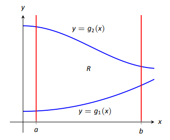
We can view the expression $\big(g_2(x)-g_1(x)\big)$ as

$$\big(g_2(x)-g_1(x)\big) = \int_{g_1(x)}^{g_2(x)} 1 \,dy =\int_{g_1(x)}^{g_2(x)} \,dy,\nonumber$$

meaning we can express the area of $R$ as an iterated integral:

$$\text{area of }R = \int_a^b \big(g_2(x)-g_1(x)\big) \,dx = \int_a^b\left(\int_{g_1(x)}^{g_2(x)} \,dy\right) \,dx =\int_a^b\int_{g_1(x)}^{g_2(x)} \,dy \,dx.$$

In short: a certain iterated integral can be viewed as giving the area of a plane region.

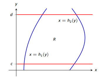
A region $R$ could also be defined by $c\leq y\leq d$ and $h_1(y)\leq x\leq h_2(y)$, as shown in Figure $\PageIndex{2}$. Using a process similar to that above, we have
$$\text{the area of }R = \int_c^d\int_{h_1(y)}^{h_2(y)} \,dx \,dy.$$

Figure $\PageIndex{2}$: Calculating the area of a plane region R with an iterated integral.

We state this formally in a theorem.

THEOREM $\PageIndex{1}$: Area of a plane region

1. Let $R$ be a plane region bounded by $a\leq x\leq b$ and $g_1(x)\leq y\leq g_2(x)$, where $g_1$ and $g_2$ are continuous functions on $[a,b]$. The area $A$ of $R$ is $$A = \int_a^b\int_{g_1(x)}^{g_2(x)} \,dy \,dx.$$
2. Let $R$ be a plane region bounded by $c\leq y\leq d$ and $h_1(y)\leq x\leq h_2(y)$, where $h_1$ and $h_2$ are continuous functions on $[c,d]$. The area $A$ of $R$ is $$A = \int_c^d\int_{h_1(y)}^{h_2(y)} \,dx \,dy.$$

The following examples should help us understand this theorem.

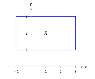
Example $\PageIndex{4}$: Area of a rectangle

Find the area $A$ of the rectangle with corners $(-1,1)$ and $(3,3)$, as shown in Figure $\PageIndex{3}$.

Figure $\PageIndex{3}$: Calculating the area of a rectangle with an iterated integral in Example $\PageIndex{4}$.

Solution

Multiple integration is obviously overkill in this situation, but we proceed to establish its use.

The region $R$ is bounded by $x=-1$, $x=3$, $y=1$ and $y=3$. Choosing to integrate with respect to $y$ first, we have
$$A = \int_{-1}^3\int_1^3 1 \,dy \,dx = \int_{-1}^3 \left(y\ \Big|_1^3\right) \,dx = \int_{-1}^3 2 \,dx = 2x\Big|_{-1}^3=8.\nonumber$$

We could also integrate with respect to $x$ first, giving:
$$A = \int_1^3\int_{-1}^3 1 \,dx \,dy =\int_1^3 \left(x\ \Big|_{-1}^3\right) \,dy = \int_1^3 4 \,dy = 4y\Big|_1^3 = 8.\nonumber$$

Clearly there are simpler ways to find this area, but it is interesting to note that this method works.

Example $\PageIndex{5}$: Area of a triangle

Find the area $A$ of the triangle with vertices at $(1,1)$, $(3,1)$ and $(5,5)$, as shown in Figure $\PageIndex{4}$.

Figure $\PageIndex{4}$: Calculating the area of a triangle with iterated integrals in Example $\PageIndex{5}$.

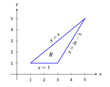
Solution

The triangle is bounded by the lines as shown in the figure. Choosing to integrate with respect to $x$ first gives that $x$ is bounded by $x=y$ to $x = \frac{y+5}2$, while $y$ is bounded by $y=1$ to $y=5$. (Recall that since $x$-values increase from left to right, the leftmost curve, $x=y$, is the lower bound and the rightmost curve, $x=(y+5)/2$, is the upper bound.) The area is

$$\begin{align*} A &= \int_1^5\int_{y}^{\frac{y+5}2} \,dx \,dy \\ &= \int_1^5\left(x\ \Big|_y^{\frac{y+5}2}\right) \,dy \\ &= \int_1^5 \left(-\frac12y+\frac52\right) \,dy \\ &= \left(-\frac14y^2+\frac52y\right)\Big|_1^5\\ &=4. \end{align*}$$

We can also find the area by integrating with respect to $y$ first. In this situation, though, we have two functions that act as the lower bound for the region $R$, $y=1$ and $y=2x-5$. This requires us to use two iterated integrals. Note how the $x$-bounds are different for each integral:

$$\begin{align*} A &= \int_1^3\int_1^x 1 \,dy \,dx &+& & &\int_3^5\int_{2x-5}^x1 \,dy \,dx\\ &= \int_1^3\big(y\big)\Big|_1^x \,dx & + & & & \int_3^5\big(y\big)\Big|_{2x-5}^x \,dx\\ &= \int_1^3\big(x-1\big) \,dx & + & & & \int_3^5\big(-x+5\big) \,dx \\ &= 2 & + & & & 2 \\ &=4. \end{align*}$$

As expected, we get the same answer both ways.

Example $\PageIndex{6}$: Area of a plane region

Find the area of the region enclosed by $y=2x$ and $y=x^2$, as shown in Figure $\PageIndex{5}$.

Figure $\PageIndex{5}$: Calculating the area of a plane region with iterated integrals in Example $\PageIndex{6}$.

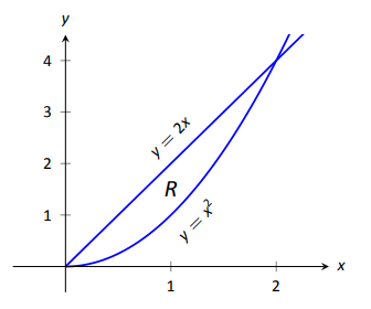
Solution

Once again we'll find the area of the region using both orders of integration.

Using $\,dy \,dx$:

$$\int_0^2\int_{x^2}^{2x}1 \,dy \,dx = \int_0^2(2x-x^2) \,dx = \big(x^2-\frac13x^3\big)\Big|_0^2 = \frac43.$$

Using $\,dx \,dy$:

$$\int_0^4\int_{y/2}^{\sqrt{y}} 1 \,dx \,dy = \int_0^4 (\sqrt{y}-y/2) \,dy = \left(\frac23y^{3/2} - \frac14y^2\right)\Big|_0^4 = \frac43.$$

Changing Order of Integration

In each of the previous examples, we have been given a region $R$ and found the bounds needed to find the area of $R$ using both orders of integration. We integrated using both orders of integration to demonstrate their equality.

We now approach the skill of describing a region using both orders of integration from a different perspective. Instead of starting with a region and creating iterated integrals, we will start with an iterated integral and rewrite it in the other integration order. To do so, we'll need to understand the region over which we are integrating.

The simplest of all cases is when both integrals are bound by constants. The region described by these bounds is a rectangle (see Example $\PageIndex{4}$), and so:

$$\int_a^b\int_c^d 1 \,dy \,dx = \int_c^d\int_a^b1 \,dx \,dy.$$

When the inner integral's bounds are not constants, it is generally very useful to sketch the bounds to determine what the region we are integrating over looks like. From the sketch we can then rewrite the integral with the other order of integration.

Examples will help us develop this skill.

Example $\PageIndex{7}$: Changing the order of integration

Rewrite the iterated integral $\displaystyle \int_0^6\int_0^{x/3} 1 \,dy \,dx$ with the order of integration $\,dx \,dy$.

Solution

We need to use the bounds of integration to determine the region we are integrating over.

The bounds tell us that $y$ is bounded by $0$ and $x/3$; $x$ is bounded by 0 and 6. We plot these four curves: $y=0$, $y=x/3$, $x=0$ and $x=6$ to find the region described by the bounds. Figure $\PageIndex{6}$ shows these curves, indicating that $R$ is a triangle.

Figure $\PageIndex{6}$: Sketching the region R described by the iterated integral in Example $\PageIndex{7}$.

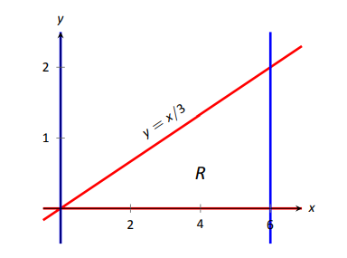
To change the order of integration, we need to consider the curves that bound the $x$-values. We see that the lower bound is $x=3y$ and the upper bound is $x=6$. The bounds on $y$ are $0$ to $2$. Thus we can rewrite the integral as $\displaystyle \int_0^2\int_{3y}^6 1 \,dx \,dy.$

Example $\PageIndex{8}$: Changing the order of integration

Change the order of integration of $\displaystyle \int_0^4\int_{y^2/4}^{(y+4)/2}1 \,dx \,dy$.

Solution

We sketch the region described by the bounds to help us change the integration order. $x$ is bounded below and above (i.e., to the left and right) by $x=y^2/4$ and $x=(y+4)/2$ respectively, and $y$ is bounded between 0 and 4. Graphing the previous curves, we find the region $R$ to be that shown in Figure $\PageIndex{7}$.

Figure $\PageIndex{7}$: Drawing the region determined by the bounds of integration in Example $\PageIndex{8}$.

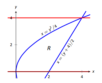
To change the order of integration, we need to establish curves that bound $y$. The figure makes it clear that there are two lower bounds for $y$: $y=0$ on $0\leq x\leq 2$, and $y=2x-4$ on $2\leq x\leq 4$. Thus we need two double integrals. The upper bound for each is $y=2\sqrt{x}$. Thus we have
$$\int_0^4\int_{y^2/4}^{(y+4)/2}1 \,dx \,dy = \int_0^2\int_0^{2\sqrt{x}} 1 \,dy \,dx + \int_2^4\int_{2x-4}^{2\sqrt{x}}1 \,dy \,dx.\nonumber$$

This section has introduced a new concept, the iterated integral. We developed one application for iterated integration: area between curves. However, this is not new, for we already know how to find areas bounded by curves.

In the next section we apply iterated integration to solve problems we currently do not know how to handle. The "real" goal of this section was not to learn a new way of computing area. Rather, our goal was to learn how to define a region in the plane using the bounds of an iterated integral. That skill is very important in the following sections.