13.4: Center of Mass

We have used iterated integrals to find areas of plane regions and signed volumes under surfaces. A brief recap of these uses will be useful in this section as we apply iterated integrals to compute the mass and center of mass of planar regions.

To find the area of a planar region, we evaluated the double integral $\displaystyle \iint_R \,dA$. That is, summing up the areas of lots of little subregions of $R$ gave us the total area. Informally, we think of $\displaystyle \iint_R \,dA$ as meaning "sum up lots of little areas over $R$.''

To find the signed volume under a surface, we evaluated the double integral $\displaystyle \iint_R f(x,y) \,dA$. Recall that the "$dA$" is not just a "bookend'' at the end of an integral; rather, it is multiplied by $f(x,y)$. We regard $f(x,y)$ as giving a height, and $dA$ still giving an area: $f(x,y) \,dA$ gives a volume. Thus, informally, $\displaystyle \iint_Rf(x,y) \,dA$ means "sum up lots of little volumes over $R$.''

We now extend these ideas to other contexts.

Mass and Weight

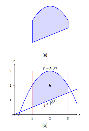
Consider a thin sheet of material with constant thickness and finite area. Mathematicians (and physicists and engineers) call such a sheet a lamina. So consider a lamina, as shown in Figure $\PageIndex{1a}$, with the shape of some planar region $R$, as shown in part (b).

Figure $\PageIndex{1}$: Illustrating the concept of a lamina.

We can write a simple double integral that represents the mass of the lamina: $\displaystyle \iint_R\ dm$, where "$dm$" means "a little mass.'' That is, the double integral states the total mass of the lamina can be found by "summing up lots of little masses over $R$.''

To evaluate this double integral, partition $R$ into $n$ subregions as we have done in the past. The $i^{\text{th}}$ subregion has area $\Delta A_i$.
A fundamental property of mass is that "mass=density$\times$area.'' If the lamina has a constant density $\delta$, then the mass of this $i^{\,\text{th}}$ subregion is $\Delta m_i=\delta\Delta A_i$. That is, we can compute a small amount of mass by multiplying a small amount of area by the density.

If density is variable, with density function $\delta= \delta(x,y)$, then we can approximate the mass of the $i^{\text{th}}$ subregion of $R$ by multiplying $\Delta A_i$ by $\delta(x_i,y_i)$, where $(x_i,y_i)$ is a point in that subregion. That is, for a small enough subregion of $R$, the density across that region is almost constant.

Note: Mass and weight are different measures. Since they are scalar multiples of each other, it is often easy to treat them as the same measure. In this section we effectively treat them as the same, as our technique for finding mass is the same as for finding weight. The density functions used will simply have different units.

The total mass $M$ of the lamina is approximately the sum of approximate masses of subregions:
$$M \approx \sum_{i=1}^n \Delta m_i = \sum_{i=1}^n \delta(x_i,y_i)\,\Delta A_i.\nonumber$$

Taking the limit as the size of the subregions shrinks to 0 gives us the actual mass; that is, integrating $\delta(x,y)$ over $R$ gives the mass of the lamina.

Definition 103 Mass of a Lamina with VarIable Density

Let $\delta(x,y)$ be a continuous density function of a lamina corresponding to a plane region $R$. The mass $M$ of the lamina is

$$\text{mass } M = \iint_R\ dm = \iint_R \delta(x,y) \,dA.$$

Example $\PageIndex{1}$: Finding the mass of a lamina with constant density

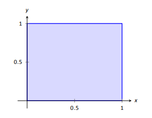
Find the mass of a square lamina, with side length 1, with a density of $\delta = 3$ gm/cm$^2$.

Solution

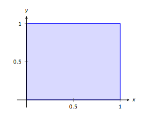
We represent the lamina with a square region in the plane as shown in Figure $\PageIndex{2}$. As the density is constant, it does not matter where we place the square.

Figure $\PageIndex{2}$: A region R representing a lamina in Example $\PageIndex{1}$.

Following Definition 103, the mass $M$ of the lamina is
$$M = \iint_R 3 \,dA = \int_0^1\int_0^1 3\, dx \, dy = 3\int_0^1\int_0^1 \, dx \, dy=3\text{ gm}.\nonumber$$

This is all very straightforward; note that all we really did was find the area of the lamina and multiply it by the constant density of $3$ gm/cm$^2$.

Example $\PageIndex{2}$: Finding the mass of a lamina with variable density

Find the mass of a square lamina, represented by the unit square with lower lefthand corner at the origin (see Figure $\PageIndex{2}$), with variable density $\delta(x,y) = (x+y+2)$ gm/cm$^2$.

Solution

The variable density $\delta$, in this example, is very uniform, giving a density of $3$ in the center of the square and changing linearly. A graph of $\delta(x,y)$ can be seen in Figure $\PageIndex{3}$; notice how "same amount'' of density is above $z=3$ as below. We'll comment on the significance of this momentarily.

The mass $M$ is found by integrating $\delta(x,y)$ over $R$. The order of integration is not important; we choose $dx \,dy$ arbitrarily. Thus:
$$\begin{align*} M = \iint_R(x+y+2) dA &= \int_0^1\int_0^1 (x+y+2)\ dx \,dy\\ &= \int_0^1\left.\left(\frac 12x^2+x(y+2)\right)\right|_0^1\,dy\\ &= \int_0^1 \left(\frac52+y\right) \,dy\\ &= \left.\left(\frac52y+\frac12y^2\right)\right|_0^1\\ &= 3\text{ gm}. \end{align*}$$

Figure $\PageIndex{3}$: Graphing the density functions in Examples $\PageIndex{1}$ and $\PageIndex{2}$.

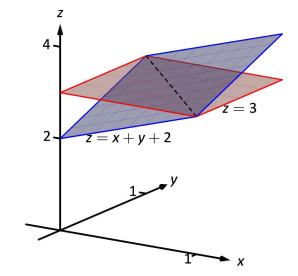
It turns out that since since the density of the lamina is so uniformly distributed "above and below'' $z=3$ that the mass of the lamina is the same as if it had a constant density of 3. The density functions in Examples $\PageIndex{1}$ and $\PageIndex{2}$ are graphed in Figure $\PageIndex{3}$, which illustrates this concept.

Example $\PageIndex{3}$: Finding the weight of a lamina with variable density

Find the weight of the lamina represented by the circle with radius $2$ ft, centered at the origin, with density function $\delta(x,y) = (x^2+y^2+1)$ lb/ft$^2$. Compare this to the weight of the same lamina with density $\delta(x,y) = (2\sqrt{x^2+y^2}+1)$ lb/ft$^2$.

Solution
A direct application of Definition 103 states that the weight of the lamina is $\displaystyle \iint_R\delta(x,y) \,dA$. Since our lamina is in the shape of a circle, it makes sense to approach the double integral using polar coordinates.

The density function $\delta(x,y) = x^2+y^2+1$ becomes $\delta(r,\theta) = (r\cos\theta)^2+(r\sin\theta)^2+1 = r^2+1$. The circle is bounded by $0\leq r\leq 2$ and $0\leq\theta\leq2\pi$. Thus the weight $W$ is:

$$\begin{align*} W &= \int_0^{2\pi}\int_0^2 (r^2+1)r\ dr\ d\theta\\ &= \int_0^{2\pi} \left.\left(\frac14r^4+\frac12r^2\right)\right|_0^2\,d\theta\\ &= \int_0^{2\pi} \left(6\right) \,d\theta\\ &= 12\pi \approx 37.70\text{ lb}. \end{align*}$$

Now compare this with the density function $\delta(x,y) = 2\sqrt{x^2+y^2}+1$. Converting this to polar coordinates gives $\delta(r,\theta) = 2\sqrt{(r\cos\theta)^2+(r\sin\theta)^2}+1 = 2r+1$. Thus the weight $W$ is:

$$\begin{align*} W &= \int_0^{2\pi}\int_0^2 (2r+1)r\ dr\ d\theta\\ &= \int_0^{2\pi} (\frac23r^3+\frac12r^2)\Big|_0^2\,d\theta\\ &= \int_0^{2\pi} \left(\frac{22}3\right)\ d\theta\\ &= \frac{44}3\pi \approx 46.08\text{ lb}. \end{align*}$$
One would expect different density functions to return different weights, as we have here. The density functions were chosen, though, to be similar: each gives a density of 1 at the origin and a density of 5 at the outside edge of the circle, as seen in Figure $\PageIndex{4}$.

Figure $\PageIndex{4}$: Graphing the density functions in $\PageIndex{3}$. In (a) is the density function $\delta (x,y)=x^2+y^2+1$; in (b) is $\delta (x,y)=2\sqrt{x^2+y^2}+1$.

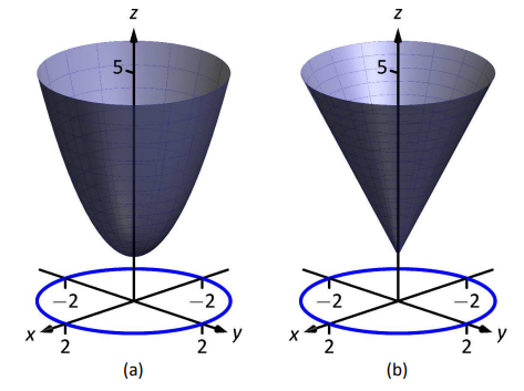
Notice how $x^2+y^2+1 \leq 2\sqrt{x^2+y^2}+1$ over the circle; this results in less weight.

Plotting the density functions can be useful as our understanding of mass can be related to our understanding of "volume under a surface.'' We interpreted $\displaystyle \iint_R f(x,y) \,dA$ as giving the volume under $f$ over $R$; we can understand $\displaystyle \iint_R\delta(x,y) \,dA$ in the same way. The "volume'' under $\delta$ over $R$ is actually mass; by compressing the "volume'' under $\delta$ onto the $xy$-plane, we get "more mass'' in some areas than others -- i.e., areas of greater density.

Knowing the mass of a lamina is one of several important measures. Another is the center of mass, which we discuss next.

Center of Mass

Consider a disk of radius 1 with uniform density. It is common knowledge that the disk will balance on a point if the point is placed at the center of the disk. What if the disk does not have a uniform density? Through trial-and-error, we should still be able to find a spot on the disk at which the disk will balance on a point. This balance point is referred to as the center of mass, or center of gravity. It is though all the mass is "centered'' there. In fact, if the disk has a mass of $3$ kg, the disk will behave physically as though it were a point-mass of $3$ kg located at its center of mass. For instance, the disk will naturally spin with an axis through its center of mass (which is why it is important to "balance'' the tires of your car: if they are "out of balance'', their center of mass will be outside of the axle and it will shake terribly).

We find the center of mass based on the principle of a weighted average. Consider a college class in which your homework average is 90%, your test average is 73%, and your final exam grade is an 85%. Experience tells us that our final grade is not the average of these three grades: that is, it is not:
$$\frac{0.9+0.73+0.85}{3} \approx 0.837 = 83.7%.\nonumber$$
That is, you are probably not pulling a B in the course. Rather, your grades are weighted. Let's say the homework is worth 10% of the grade, tests are 60% and the exam is 30%. Then your final grade is:
$$(0.1)(0.9) + (0.6)(0.73)+(0.3)(0.85) = 0.783 = 78.3%.\nonumber$$
Each grade is multiplied by a weight.

In general, given values $x_1,x_2,\ldots,x_n$ and weights $w_1,w_2,\ldots,w_n$, the weighted average of the $n$ values is
$$\sum_{i=1}^n w_ix_i\Bigg/\sum_{i=1}^n w_i.\nonumber$$

In the grading example above, the sum of the weights 0.1, 0.6 and 0.3 is 1, so we don't see the division by the sum of weights in that instance.

How this relates to center of mass is given in the following theorem.

THEOREM 121 Center of Mass of Discrete Linear System

Let point masses $m_1,m_2,\ldots,m_n$ be distributed along the $x$-axis at locations $x_1,x_2,\ldots,x_n$, respectively. The center of mass $\overline{x}$ of the system is located at

$$\overline{x} = \sum_{i=1}^nm_ix_i\Bigg/\sum_{i=1}^n m_i.$$

Example $\PageIndex{4}$: Finding the center of mass of a discrete linear system

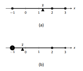
1. Point masses of $2$ gm are located at $x=-1$, $x=2$ and $x=3$ are connected by a thin rod of negligible weight. Find the center of mass of the system.
2. Point masses of $10$ gm, $2$ gm and $1$ gm are located at $x=-1$, $x=2$ and $x=3$, respectively, are connected by a thin rod of negligible weight. Find the center of mass of the system.

Solution

1. Following Theorem 121, we compute the center of mass as:
   $$\overline{x}=\frac{2(-1) + 2(2)+2(3)}{2+2+2} = \frac43 = 1.\overline{3}.$$
   So the system would balance on a point placed at $x=4/3$, as illustrated in Figure $\PageIndex{5a}$.
2. Again following Theorem 121, we find:
   $$\overline{x} = \frac{10(-1)+2(2)+1(3)}{10+2+1} = \frac{-3}{13} \approx -0.23.$$
   Placing a large weight at the left hand side of the system moves the center of mass left, as shown in Figure $\PageIndex{5b}$.

Figure $\PageIndex{5}$: Illustrating point masses along a thin rod and the center of mass.

In a discrete system (i.e., mass is located at individual points, not along a continuum) we find the center of mass by dividing the mass into a moment of the system. In general, a moment is a weighted measure of distance from a particular point or line. In the case described by Theorem 121, we are finding a weighted measure of distances from the $y$-axis, so we refer to this as the moment about the $y$-axis, represented by $M_y$. Letting $M$ be the total mass of the system, we have $\overline{x} = M_y/M$.

We can extend the concept of the center of mass of discrete points along a line to the center of mass of discrete points in the plane rather easily. To do so, we define some terms then give a theorem.

Definition 104 Moments about the $x$- and $y$- Axes.

Let point masses $m_1$, $m_2,\ldots,m_n$ be located at points $(x_1,y_1)$, $(x_2,y_2)\ldots,(x_n,y_n)$, respectively, in the $xy$-plane.

1. The moment about the $y$-axis, $M_y$, is $\displaystyle M_y = \sum_{i=1}^n m_ix_i.$
2. The moment about the $x$-axis}, $M_x$, is $\displaystyle M_x = \sum_{i=1}^n m_iy_i.$

One can think that these definitions are "backwards'' as $M_y$ sums up "$x$" distances. But remember, "$x$" distances are measurements of distance from the $y$-axis, hence defining the moment about the $y$-axis.

We now define the center of mass of discrete points in the plane.

THEOREM 122 Center of Mass of Discrete Planar System

Let point masses $m_1$, $m_2,\ldots,m_n$ be located at points $(x_1,y_1)$, $(x_2,y_2)\ldots,(x_n,y_n)$, respectively, in the $xy$-plane, and let $\displaystyle M = \sum_{i=1}^n m_i$.
The center of mass of the system is at $(\overline{x},\,\overline{y})$, where
$$\overline{x}= \frac{M_y}{M}\quad \text{and}\quad \overline{y} = \frac{M_x}{M}.$$

Example $\PageIndex{5}$: Finding the center of mass of a discrete planar system

Let point masses of $1$ kg, $2$ kg and $5$ kg be located at points $(2,0)$, $(1,1)$ and $(3,1)$, respectively, and are connected by thin rods of negligible weight. Find the center of mass of the system.

Solution

We follow Theorem 122 and Definition 104 to find $M$, $M_x$ and $M_y$:

$M = 1+2+5 = 8$kg.
$$\begin{align*} M_x &= \sum_{i=1}^n m_iy_i \\ &= 1(0) + 2(1) + 5(1) \\ &= 7. \end{align*}$$

$$\begin{align*} M_y &= \sum_{i=1}^n m_ix_i \\ &= 1(2) + 2(1) + 5(3) \\ &= 19. \end{align*}$$

Figure $\PageIndex{6}$: Illustrating the center of mass of a discrete planar system in Example $\PageIndex{5}$.

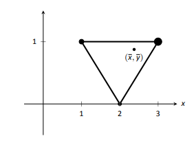
Thus the center of mass is $(\overline{x},\,\overline{y}) = \left(\frac{M_y}{M},\frac{M_x}M\right) = \left(\frac198,\frac78\right) =(2.375,0.875),$ illustrated in Figure $\PageIndex{6}$.

We finally arrive at our true goal of this section: finding the center of mass of a lamina with variable density. While the above measurement of center of mass is interesting, it does not directly answer more realistic situations where we need to find the center of mass of a contiguous region. However, understanding the discrete case allows us to approximate the center of mass of a planar lamina; using calculus, we can refine the approximation to an exact value.

We begin by representing a planar lamina with a region $R$ in the $xy$-plane with density function $\delta(x,y)$. Partition $R$ into $n$ subdivisions, each with area $\Delta A_i$. As done before, we can approximate the mass of the $i^{\text{th}}$ subregion with $\delta(x_i,\,y_i)\,\Delta A_i$, where $(x_i,\,y_i)$ is a point inside the $i^{\text{th}}$ subregion. We can approximate the moment of this subregion about the $y$-axis with $x_i\,\delta(x_i,y_i)\,\Delta A_i$ -- that is, by multiplying the approximate mass of the region by its approximate distance from the $y$-axis. Similarly, we can approximate the moment about the $x$-axis with $y_i\,\delta(x_i,y_i)\,\Delta A_i$. By summing over all subregions, we have:

$$\begin{align*} \text{mass: } M &\approx \sum_{i=1}^n \delta(x_i,y_i)\,\Delta A_i\quad \text{(as seen before)}\\ \text{moment about the \(x\)-axis: } M_x &\approx \sum_{i=1}^n y_i\delta(x_i,y_i)\,\Delta A_i\\ \text{moment about the \(y\)-axis: } M_y &\approx \sum_{i=1}^n x_i\delta(x_i,y_i)\,\Delta A_i\\ \end{align*}$$

By taking limits, where size of each subregion shrinks to 0 in both the $x$ and $y$ directions, we arrive at the double integrals given in the following theorem.

Theorem 123: Center of Mass of a Planar Lamina, Moments

Let a planar lamina be represented by a region $R$ in the $xy$-plane with density function $\delta(x,y)$.

1. $\displaystyle \text{mass: } M = \iint_R\delta(x,y) \,dA$
2. $\displaystyle \text{moment about the \(x\)-axis: } M_x = \iint_Ry\delta(x,y) \,dA$
3. $\displaystyle \text{moment about the \(y\)-axis: } M_y = \iint_Rx\delta(x,y) \,dA$
4. The center of mass of the lamina is
   $$(\overline{x},\,\overline{y}) = \left(\frac{M_y}{M},\frac{M_x}M\right).\nonumber$$

We start our practice of finding centers of mass by revisiting some of the lamina used previously in this section when finding mass. We will just set up the integrals needed to compute $M$, $M_x$ and $M_y$ and leave the details of the integration to the reader.

Example $\PageIndex{6}$: Finding the center of mass of a lamina

Find the center mass of a square lamina, with side length 1, with a density of $\delta = 3$ gm/cm$^2$. (Note: this is the lamina from Example $\PageIndex{1}$.)

Solution
We represent the lamina with a square region in the plane as shown in Figure $\PageIndex{7}$ as done previously.

Figure $\PageIndex{7}$: A region R representing a lamina in Example $\PageIndex{6}$.

Following Theorem 123, we find $M$, $M_x$ and $M_y$:

$$\begin{align*} M &= \iint_R 3 \,dA = \int_0^1\int_0^1 3\ dx \,dy =3\text{ gm}.\\ M_x &= \iint_R 3y \,dA = \int_0^1\int_0^1 3y\ dx\, dy =3/2 = 1.5.\\ M_y &= \iint_R 3x \,dA = \int_0^1\int_0^1 3x\ dx \,dy =3/2 = 1.5. \end{align*}$$

Thus the center of mass is $(\overline{x},\,\overline{y}) = \left(\frac{M_y}M,\frac{M_x}M\right) = (1.5/3,1.5/3) = (0.5,0.5).$ This is what we should have expected: the center of mass of a square with constant density is the center of the square.

Example $\PageIndex{7}$: Finding the center of mass of a lamina

Find the center of mass of a square lamina, represented by the unit square with lower left-hand corner at the origin (see Figure $\PageIndex{7}$), with variable density $\delta(x,y) = (x+y+2)$ gm/cm$^2$. (Note: this is the lamina from Example $\PageIndex{2}$.)

Solution
We follow Theorem 123, to find $M$, $M_x$ and $M_y$:

$$\begin{align*} M &= \iint_R (x+y+2) \,dA = \int_0^1\int_0^1 (x+y+2)\ dx \,dy =3\text{ gm}.\\ M_x &= \iint_R y(x+y+2) \,dA = \int_0^1\int_0^1 y(x+y+2)\ dx \,dy =\frac{19}{12}.\\ M_y &= \iint_R x(x+y+2) \,dA = \int_0^1\int_0^1 x(x+y+2)\ dx \,dy =\frac{19}{12}. \end{align*}$$

Thus the center of mass is $(\overline{x},\overline{y}) = \left(\frac{M_y}M,\frac{M_x}M\right) = \left(\frac{19}{36},\frac{19}{36}\right) \approx (0.528,0.528).$ While the mass of this lamina is the same as the lamina in the previous example, the greater density found with greater $x$ and $y$ values pulls the center of mass from the center slightly towards the upper right-hand corner.

Example $\PageIndex{8}$: Finding the center of mass of a lamina

Find the center of mass of the lamina represented by the circle with radius $2$ ft, centered at the origin, with density function $\delta(x,y) = (x^2+y^2+1)$ lb/ft$^2$. (Note: this is one of the lamina used in Example $\PageIndex{3}$.)

Solution

As done in Example $\PageIndex{3}$, it is best to describe $R$ using polar coordinates.
Thus when we compute $M_y$, we will integrate not $x\delta(x,y) = x(x^2+y^2+1)$, but rather $\big(r\cos\theta\big)\delta(r\cos\theta,r\sin\theta) = \big(r\cos\theta\big)\big(r^2+1\big).$ We compute $M$, $M_x$ and $M_y$:

$$\begin{align*} M &= \int_0^{2\pi}\int_0^2 (r^2+1)r\ dr\ d\theta = 12\pi\approx 37.7\text{ lb}.\\ M_x &= \int_0^{2\pi}\int_0^2 (r\sin\theta)(r^2+1)r \ dr\ d\theta = 0.\\ M_y &= \int_0^{2\pi}\int_0^2 (r\cos\theta)(r^2+1)r \ dr\ d\theta = 0.\\ \end{align*}$$

Since $R$ and the density of $R$ are both symmetric about the $x$ and $y$ axes, it should come as no big surprise that the moments about each axis is $0.$ Thus the center of mass is $(\overline{x},\,\overline{y})=(0,0)$.

Example $\PageIndex{9}$: Finding the center of mass of a lamina

Find the center of mass of the lamina represented by the region $R$ shown in Figure $\PageIndex{8}$, half an annulus with outer radius 6 and inner radius 5, with constant density $2$ lb/ft$^{2}$.

Solution

Once again it will be useful to represent $R$ in polar coordinates. Using the description of $R$ and/or the illustration, we see that $R$ is bounded by $5\leq r\leq 6$ and $0\leq\theta\leq\pi$. As the lamina is symmetric about the $y$-axis, we should expect $M_y=0$. We compute $M$, $M_x$ and $M_y$:
$$\begin{align*} M &= \int_0^{\pi}\int_5^6 (2)r\ dr\ d\theta = 11\pi\text{ lb}.\\ M_x &= \int_0^{\pi}\int_5^6 (r\sin\theta)(2)r\ dr\ d\theta = \frac{364}3\approx 121.33 .\\ M_y &= \int_0^{\pi}\int_5^6 (r\cos\theta)(2)r\ dr\ d\theta = 0.\\ \end{align*}$$

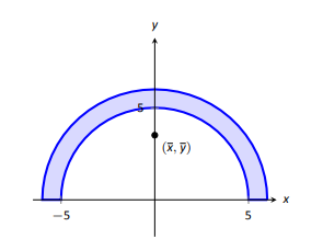
Figure $\PageIndex{8}$: Illustrating the region $R$ in Example $\PageIndex{9}$.

Thus the center of mass is $(\overline{x},\,\overline{y}) = \left(0,\frac{364}{33\pi}\right) \approx (0,\,3.51).$ The center of mass is indicated in Figure $\PageIndex{8}$; note how it lies outside of $R$!

This section has shown us another use for iterated integrals beyond finding area or signed volume under the curve. While there are many uses for iterated integrals, we give one more application in the following section: computing surface area.