8.6: Numerical Integration

We have now seen some of the most generally useful methods for discovering antiderivatives, and there are others. Unfortunately, some functions have no simple antiderivatives; in such cases if the value of a definite integral is needed it will have to be approximated. We will see two methods that work reasonably well and yet are fairly simple; in some cases more sophisticated techniques will be needed.

Of course, we already know one way to approximate an integral: if we think of the integral as computing an area, we can add up the areas of some rectangles. While this is quite simple, it is usually the case that a large number of rectangles is needed to get acceptable accuracy. A similar approach is much better: we approximate the area under a curve over a small interval as the area of a trapezoid. In figure \(\PageIndex{1}\) we see an area under a curve approximated by rectangles and by trapezoids; it is apparent that the trapezoids give a substantially better approximation on each subinterval.

 

 

Figure \(\PageIndex{1}\). Approximating an area with rectangles and with trapezoids.

As with rectangles, we divide the interval into \(n\) equal subintervals of length \(\Delta x\). A typical trapezoid is pictured in figure \(\PageIndex{2}\); it has area \(\dfrac{f(x_i)+f(x_{i+1})}{2}\Delta x\). If we add up the areas of all the trapezoids, we get \[\eqalign{{f(x_0)+f(x_1)\over 2}\Delta x&+{f(x_1)+f(x_2)\over 2}\Delta x+\cdots+{f(x_{n-1})+f(x_n)\over 2}\Delta x=\cr&\left({f(x_0)\over 2}+f(x_1)+f(x_2)+\cdots+f(x_{n-1})+{f(x_n)\over 2}\right)\Delta x.\cr}\nonumber\]

This is usually known as the Trapezoid Rule. For a modest number of subintervals this is not too difficult to do with a calculator; a computer can easily do many subintervals.

Figure \(\PageIndex{2}\). A single trapezoid.

In practice, an approximation is useful only if we know how accurate it is; for example, we might need a particular value accurate to three decimal places. When we compute a particular approximation to an integral, the error is the difference between the approximation and the true value of the integral. For any approximation technique, we need an error estimate, a value that is guaranteed to be larger than the actual error. If \(A\) is an approximation and \(E\) is the associated error estimate, then we know that the true value of the integral is between \(A-E\) and \(A+E\). In the case of our approximation of the integral, we want \(E=E(\Delta x)\) to be a function of \(\Delta x\) that gets small rapidly as \(\Delta x\) gets small. Fortunately, for many functions, there is such an error estimate associated with the trapezoid approximation.

Theorem \(\PageIndex{1}\)

Suppose \(f\) has a second derivative \(f''\) everywhere on the interval \([a,b]\), and \(|f''(x)|\le M\) for all \(x\) in the interval. With \(\Delta x=(b-a)/n\), an error estimate for the trapezoid approximation is \[E(\Delta x) = {b-a\over 12}M(\Delta x)^2={(b-a)^3\over 12n^2}M.\nonumber\]

Let's see how we can use this.

Example \(\PageIndex{2}\)

Approximate \(\displaystyle\int_0^1 e^{−x^2}\,dx\) to two decimal places.

Solution

The second derivative of \(f(x)=e^{−x^2}\) is \((4x^2−2)e^{−x^2}\), and it is not hard to see that on \([0,1]\), \(|(4x^2−2)e^{−x^2}|\le 2\). We begin by estimating the number of subintervals we are likely to need. To get two decimal places of accuracy, we will certainly need \(E(\Delta x)<0.005\) or

\[\eqalign{\dfrac{1}{12}\times(2)\times\dfrac{1}{n^2}&\lt 0.005\cr\dfrac{1}{6}\times 200&\lt n^2\cr 5.77\approx\sqrt{\dfrac{100}{3}}&\lt n\cr}\nonumber\]

With \(n=6\), the error estimate is thus \(\dfrac{1}{6\cdot 6^2}\lt 0.0047\). We compute the trapezoid approximation for six intervals: \[\left(\dfrac{f(0)}{2}+f(1/6)+f(2/6)+\cdots+f(5/6)+\dfrac{f(1)}{2}\right)\dfrac{1}{6}\approx 0.74512.\nonumber\]

So the true value of the integral is between \(0.74512−0.0047=0.74042\) and \(0.74512+0.0047=0.74982\). Unfortunately, the first rounds to \(0.74\) and the second rounds to \(0.75\), so we can't be sure of the correct value in the second decimal place; we need to pick a larger \(n\). As it turns out, we need to go to \(n=12\) to get two bounds that both round to the same value, which turns out to be \(0.75\). For comparison, using \(12\) rectangles to approximate the area gives \(0.7727\), which is considerably less accurate than the approximation using six trapezoids.

In practice it generally pays to start by requiring better than the maximum possible error; for example, we might have initially required \(E(\Delta x)<0.001\), or
\[\eqalign{\dfrac{1}{12}\times(2)\times\dfrac{1}{n^2}&\lt 0.001\cr\dfrac{1}{6}\times 1000&\lt n^2\cr 12.91\approx\sqrt{\dfrac{500}{3}}&\lt n.\cr}\nonumber\]
Had we immediately tried \(n=13\), this would have given us the desired answer.

The trapezoid approximation works well, especially compared to rectangles, because the tops of the trapezoids form a reasonably good approximation to the curve when \(\Delta x\) is fairly small. We can extend this idea: what if we try to approximate the curve more closely, by using something other than a straight line? The obvious candidate is a parabola: if we can approximate a short piece of the curve with a parabola with equation \(y=ax^2+bx+c\), we can easily compute the area under the parabola.

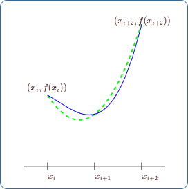
There are an infinite number of parabolas through any two given points, but only one through three given points. If we find a parabola through three consecutive points \((x_i,f(x_i))\), \((x_{i+1},f(x_{i+1}))\), \((x_{i+2},f(x_{i+2}))\) on the curve, it should be quite close to the curve over the whole interval \([x_i,x_{i+2}]\), as in figure \(\PageIndex{3}\). If we divide the interval \([a,b]\) into an even number of subintervals, we can then approximate the curve by a sequence of half as many parabolas, each one covering two of the subintervals.

For this to be practical, we would like a (hopefully simple) formula for the area of two consecutive subintervals under the parabola \(ax^2+bx+c\), which passes through \((x_i,f(x_i))\), \((x_{i+1},f(x_{i+1}))\), and \((x_{i+2},f(x_{i+2}))\). One way to discover this formula (below) in terms of the \(x\)'s and \(f\)'s without knowing it in advance, would be to first use the three pairs of \(x,f\) values lying on the parabola to solve the resulting simultaneous linear equations to get expressions for \(a, b,\) and \(c\), and then using those to find the area by integrating the quadratic over the width of the two subintervals. Although the algebra to do this is quite possible and straightforward in principle, it is long and involves a lot of detail, so it is remarkable how well the final result simplifies at the end of the computation. However, once the formula for the area of two subintervals is known, much less algebra is needed just to prove that it is correct, as in that case it's only necessary to leave \(a, b,\) and \(c\) in the proof as they are, without having to first solve for them in terms of the \(x\)'s and \(f\)'s. The algebra is well within the capability of a good computer algebra system, and we will just present the result. The integral for the area of two consecutive equal width \(\Delta x\) subintervals centered on \(x_{i+1}\) turns out to be: \[\int_{x_{i+1}-\Delta x}^{x_{i+1}+\Delta x}(ax^2+bx+c)\,dx= 2\Delta x\times\dfrac{(f(x_i)+4f(x_{i+1})+f(x_{i+2}))}{6}.\nonumber\]

This area is, of course, \((\)width \(2\Delta x)\times(\)height\()\), where instead of taking the average height equally of the three values of \(f\), which would be \(\dfrac{2f(x_i)+2f(x_{i+1})+2f(x_{i+2})}{6}\), the central value \(f(x_{i+1})\) counts as contributing double in "weight" to the total while the contributions of the two outer values are correspondingly halved. Given that the interpolation has introduced a curve, the parabola, the resulting expression for the area integral could hardly be any simpler.

Once this formula for the area of one pair of adjacent subintervals is known, the sum of the areas under all the parabolas for all of the pairs of subintervals is easily seen to be \[\displaylines{{\Delta x\over 3}\left(\;\big(f(x_0)+4f(x_{1})+f(x_{2})\big)\;+\;\big(f(x_2)+4f(x_{3})+f(x_{4})\big)\;+\cdots+\;\big(f(x_{n-2})+4f(x_{n-1})+f(x_{n})\big)\;\right)=\cr{\Delta x\over 3}\big(f(x_0)+4f(x_{1})+2f(x_{2})+4f(x_{3})+2f(x_{4})+\cdots +2f(x_{n-2})+4f(x_{n-1})+f(x_{n})\big).\cr}\nonumber\]

This is just slightly more complicated than the formula for trapezoids; we need to remember the alternating 2 and 4 coefficients, except for the first and last values of \(f\). This approximation technique is referred to as Simpson's Rule.

Figure \(\PageIndex{3}\). A parabola (dashed) approximating a curve (solid).

As with the trapezoid method, this is useful only with an error estimate:

Theorem \(\PageIndex{3}\): Simpson error approximation

Suppose \(f\) has a fourth derivative \(f^{(4)}\) everywhere on the interval \([a,b]\), and \(|f^{(4)}(x)|\le M\) for all \(x\) in the interval. With \(\Delta x=(b-a)/n\), an error estimate for Simpson's approximation is \[E(\Delta x) = {b-a\over 180}M(\Delta x)^4={(b-a)^5\over 180n^4}M.\nonumber\]

Example \(\PageIndex{4}\)

Let us again approximate \(\displaystyle\int_0^1 e^{−x^2}\,dx\) to two decimal places.

Solution

The fourth derivative of \(f=e^{−x^2}\) is \((16x^4−48x^2+12)e^{−x^2}\); on \([0,1]\) this is at most \(12\) in absolute value. We begin by estimating the number of subintervals we are likely to need. To get two decimal places of accuracy, we will certainly need \(E(\Delta x)\lt 0.005\), but taking a cue from our earlier example, let's require \(E(\Delta x)\lt 0.001\): \[\eqalign{\dfrac{1}{180}\times(12)\times\dfrac{1}{n^4}&\lt 0.001\cr\dfrac{200}{3}&\lt n^4\cr 2.86\approx\sqrt[4]{\dfrac{200}{3}}&\lt n.\cr}\nonumber\]

So we try \(n=4\), since we need an even number of subintervals. Then the error estimate is \(\dfrac{12}{180\times 4^4}<0.0003\), and the approximation is \[\dfrac{0.25}{3}\times\big(f(0)+4f(0.25)+2f(0.5)+4f(0.75)+f(1)\big)\approx 0.746855.\nonumber\]

So the true value of the integral is between \(0.746855−0.0003=0.746555\) and \(0.746855+0.0003=0.747155\), both of which round to \(0.75\).

Figure \(\PageIndex{4}\) below compares the three methods we have discussed, computing the area under \(y=\sin x, 0\le x\le\pi/2\). Of course, it's easy to compute this exactly: the area is \(1\).

 

Exercises \(\PageIndex{}\)

In the following problems, compute the trapezoid and Simpson approximations using 4 subintervals, and compute the error estimate for each. (Finding the maximum values of the second and fourth derivatives can be challenging for some of these; you may use a graphing calculator or computer software to estimate the maximum values.) If you have access to Sage or similar software, approximate each integral to two decimal places.

Exercise \(\PageIndex{1}\)

\(\displaystyle\int_1^3 x\,dx\)

Answer

Trapezoid: \(4\pm 0.\quad\) Simpson: also \(4\pm 0\).

Exercise \(\PageIndex{2}\)

\(\displaystyle\int_0^3 x^2\,dx\)

Answer

Trapezoid: \(9.28125\pm 0.28125.\quad\) Simpson: \(9\pm 0\).

Exercise \(\PageIndex{3}\)

\(\displaystyle\int_2^4 x^3\,dx\)

Answer

Trapezoid: \(60.75\pm 1.\quad\) Simpson: \(60\pm 0\).

Exercise \(\PageIndex{4}\)

\(\displaystyle\int_1^3{1\over x}\,dx\)

Answer

Trapezoid: \(1.11667\pm 0.08333.\quad\) Simpson: \(1.1\pm 0.01667\).

Exercise \(\PageIndex{5}\)

\(\displaystyle\int_1^2{1\over 1+x^2}\,dx\)

Answer

Trapezoid: \(0.32352\pm 0.0026.\quad\) Simpson: \(0.32175\pm 0.000065\).

Exercise \(\PageIndex{6}\)

\(\displaystyle\int_0^1 x\sqrt{1+x}\,dx\)

Answer

Trapezoid: \(0.64779\pm 0.0052.\quad\) Simpson: \(0.64380\pm 0.000033\).

Exercise \(\PageIndex{7}\)

\(\displaystyle\int_1^5{x\over 1+x}\,dx\)

Answer

Trapezoid: \(2.88333\pm 0.0834.\quad\) Simpson: \(2.90000\pm 0.0167\).

Exercise \(\PageIndex{8}\)

\(\displaystyle\int_0^1\sqrt{x^3+1}\,dx\)

Answer

Trapezoid: \(1.11699\pm 0.0077.\quad\) Simpson: \(1.11186\pm 0.0002\).

Exercise \(\PageIndex{9}\)

\(\displaystyle\int_0^1\sqrt{x^4+1}\,dx\)

Answer

Trapezoid: \(1.09680\pm 0.0147.\quad\) Simpson: \(1.08941\pm 0.0003\).

Exercise \(\PageIndex{10}\)

\(\displaystyle\int_1^4\sqrt{1+{1\over x}}\,dx\)

Answer

Trapezoid: \(3.63484\pm 0.087.\quad\) Simpson: \(3.62178\pm 0.032\).

Exercise \(\PageIndex{11}\)

Using Simpson's rule on a parabola \(f(x)\), even with just two subintervals, gives the exact value of the integral, because the parabolas used to approximate \(f\) will be \(f\) itself. Remarkably, Simpson's rule also computes the integral of a cubic function \(f(x)=ax^3+bx^2+cx+d\) exactly. Show this is true by showing that \[\int_{x_0}^{x_2}f(x)\,dx=(x_2-x_0)\left(\dfrac{f(x_0)+4f((x_0+x_2)/2)+f(x_2)}{6}\right).\nonumber\] Hint: Do not try to determine the cubic by solving for \(a, b, c, d\) in terms of \(x_0, x_2, f(x_0), f((x_0+x_2)/2)\) and \(f(x_2)\). This isn't necessary, nor (unlike the quadratic case) is it even possible. You only need the area under the cubic, i.e. the integral, not the actual cubic itself.

Contributors

David Guichard (Whitman College)

• Integrated by Justin Marshall.