9.8: Probability

You perhaps have at least a rudimentary understanding of discrete probability, which measures the likelihood of an "event" when there are a finite number of possibilities. For example, when an ordinary six-sided die is rolled, the probability of getting any particular number is \(1/6\). In general, the probability of an event is the number of ways the event can happen divided by the number of ways that "anything" can happen.

For a slightly more complicated example, consider the case of two six-sided dice. The dice are physically distinct, which means that rolling a 2--5 is different than rolling a 5--2; each is an equally likely event out of a total of 36 ways the dice can land, so each has a probability of \(1/36\).

Most interesting events are not so simple. More interesting is the probability of rolling a certain sum out of the possibilities 2 through 12. It is clearly not true that all sums are equally likely: the only way to roll a 2 is to roll 1--1, while there are many ways to roll a 7. Because the number of possibilities is quite small, and because a pattern quickly becomes evident, it is easy to see that the probabilities of the various sums are: \[\eqalign{P(2) =P(12) &=1/36\cr P(3) = P(11) &= 2/36\cr P(4) =P(10) &= 3/36\cr P(5) =P(9) &= 4/36\cr P(6) =P(8) &= 5/36\cr P(7) &=6/36\cr}\nonumber\] Here we use \(P(n)\) to mean "the probability of rolling an \(n\)". Since we have correctly accounted for all possibilities, the sum of all these probabilities is \(36/36=1\); the probability that the sum is one of \(2\) through \(12\) is \(1\), because there are no other possibilities.

The study of probability is concerned with more difficult questions as well; for example, suppose the two dice are rolled many times. On the average, what sum will come up? In the language of probability, this average is called the expected value of the sum. This is at first a little misleading, as it does not tell us what to "expect" when the two dice are rolled, but instead it tells us what we expect the long term average will be.

Suppose that two dice are rolled 36 million times. Based on the probabilities, we would expect about 1 million rolls to be 2, about 2 million to be 3, and so on, with a roll of 7 topping the list at about 6 million. The sum of all rolls would be 1 million times 2 plus 2 million times 3, and so on, and dividing by 36 million we would get the average:

\[\eqalign{ \bar x&= (2\cdot 10^6+3(2\cdot 10^6) +\cdots+7(6\cdot 10^6)+\cdots+12\cdot10^6) {1\over 36\cdot 10^6}\cr &= 2{10^6\over 36\cdot 10^6}+3{2\cdot 10^6\over 36\cdot 10^6}+\cdots+ 7{6\cdot 10^6\over 36\cdot 10^6}+\cdots+12{10^6\over 36\cdot 10^6}\cr &=2P(2)+3P(3)+\cdots+7P(7)+\cdots+12P(12)\cr &=\sum_{i=2}^{12} iP(i)=7.}\nonumber\]

There is nothing special about the \(36\) million in this calculation. No matter what the number of rolls, once we simplify the average, we get the same \(\displaystyle\sum_{i=2}^{12}iP(i)\). While the actual average value of a large number of rolls will not be exactly \(7\), the average should be close to \(7\) when the number of rolls is large. Turning this around, if the average is not close to \(7\), we should suspect that the dice are not fair.

A variable, say \(X\), that can take certain values, each with a corresponding probability, is called a random variable; in the example above, the random variable was the sum of the two dice. Typically, the range of a random variable, i.e. all the values that it can possibly take, is a subset of the real numbers. If the possible values for \(X\) are \(x_1\), \(x_2,…,\) \(x_n\), then the expected value of the random variable is \(\displaystyle E(X)=\sum_{i=1}^n x_iP(x_i)\). The expected value is also called the mean.

When the number of possible values for \(X\) is finite, we say that \(X\) is a discrete random variable. In many applications of probability, the number of possible values of a random variable is very large, perhaps even infinite. To deal with the infinite case we need a different approach, and since there is a sum involved, it should not be wholly surprising that integration turns out to be a useful tool. It then turns out that even when the number of possibilities is large but finite, it is frequently easier to pretend that the number is infinite. Suppose, for example, that a dart is thrown at a dart board. Since the dart board consists of a finite number of atoms, there is in some sense only a finite number of places for the dart to land, but it is easier to explore the probabilities involved by pretending that the dart can land on any point in the usual (real number) \(x\)-\(y\) plane.

Definition: \(\PageIndex{1}\)

Let \(f:\mathbb{R} \to \mathbb{R}\) be a function. If \(f(x) \ge 0\) for every \(x\) and \(\displaystyle\int_{-\infty }^\infty f(x)\,dx = 1\) then \(f\) is a probability density function.

We associate a probability density function with a (real number) random variable \(X\) by stipulating that the probability that \(X\) is between \(a\) and \(b\) is \[\int_a^b f(x)\,dx.\nonumber\] Because of the requirement that the integral from \(-\infty\) to \(\infty\) be \(1\) and that \(f\) is non-negative everywhere, all probabilities are less than or equal to \(1\), and the probability that \(X\) takes on some value between \(-\infty\) and \(\infty\) is \(1\), as it should be.

Example \(\PageIndex{2}\)

Consider again the two dice example; we can view it in a way that more resembles the probability density function approach. Consider a random variable \(X\) that takes on any real value with probabilities given by the probability density function in Figure \(\PageIndex{1}\). The function \(f\) consists of just the top edges of the rectangles, with vertical sides drawn for clarity; the function is zero below \(1.5\) and above \(12.5\). The area of each rectangle is the probability of rolling the sum in the middle of the bottom of the rectangle, or \[P(n) = \int_{n-1/2}^{n+1/2}f(x)\,dx.\nonumber\] The probability of rolling a 4, 5, or 6 is \[P(n)=\int_{7/2}^{13/2}f(x)\,dx.\nonumber\] Of course, we could also compute probabilities that don't make sense in the context of the dice, such as the probability that \(X\) is between \(4\) and \(5.8\).

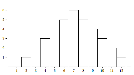
Figure \(\PageIndex{1}\). A probability density function for two dice.

The function \[F(x) = P(X\le x) = \int_{-\infty }^x f(t) dt\nonumber\] is called the cumulative distribution function, or simply the (probability) distribution.

Example \(\PageIndex{3}\)

Suppose that \(a < b\) and \[ f(x)=\cases{\dfrac{1}{b-a}& if $a\le x \le b$\cr 0&otherwise.\cr}\nonumber\] Then \(f(x)\) is the uniform probability density function on \([a,b]\), and the corresponding cumulative distribution is the uniform distribution on \([a,b]\).

Example \(\PageIndex{4}\)

Consider the function \(f(x) = e^{-{x^2}/2}\). What can we say about \[\int_{-\infty }^\infty e^{-{x^2}/2}\,dx?\nonumber\]

Solution

We cannot find an antiderivative of \(f\), but we can see that this integral is some finite number. Notice that \(0\lt f(x) = e^{-{x^2}/2}\le e^{-x/2}\) for \(|x|\gt 1\). This implies that the area under \(e^{-{x^2}/2}\) is less than the area under \(e^{-x/2}\), over the interval \([1,\infty)\). It is easy to compute the latter area, namely \[\int_1^\infty e^{-x/2}\,dx = \dfrac{2}{\sqrt{e}},\nonumber\] so \[\int_1^\infty e^{-{x^2}/2}\,dx\nonumber\] is some finite number smaller than \(2/\sqrt{e}\). Because \(f\) is symmetric around the \(y\)-axis, \[\int_{-\infty}^{-1} e^{-{x^2}/2}\,dx=\int_1^\infty e^{-{x^2}/2}\,dx.\nonumber\] This means that \[\int_{-\infty }^\infty e^{-{x^2}/2}\,dx =\int_{-\infty}^{-1} e^{-{x^2}/2}\,dx + \int_{-1}^1 e^{-{x^2}/2}\,dx + \int_1^\infty e^{-{x^2}/2}\,dx = A\nonumber\] for some finite positive number \(A\). Now if we let \(g(x) = f(x)/A\), \[ \int_{-\infty }^\infty g(x)\,dx = {1\over A}\int_{-\infty }^\infty e^{-{x^2}/2}\,dx = {1\over A} A = 1,\nonumber\] so \(g\) is a probability density function. It turns out to be very useful, and is called the standard normal probability density function or more informally the bell curve, giving rise to the standard normal distribution. See Figure \(\PageIndex{2}\) for the graph of the bell curve.

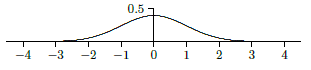
Figure \(\PageIndex{2}\). The bell curve.

We have shown that \(A\) is some finite number without computing it; we cannot compute it with the techniques we have available. By using some techniques from multivariable calculus, it can be shown that \(A=\sqrt{2\pi}\).

Example \(\PageIndex{5}\)

The exponential distribution has probability density function \[f(x) =\begin{cases} 0 & x < 0 \\ ce^{-cx } & x\ge 0 \end{cases}\nonumber\] where \(c\) is a positive constant.

The mean or expected value of a random variable is quite useful, as hinted at in our discussion of dice. Recall that the mean for a discrete random variable is \(\displaystyle E(X)=\sum_{i=1}^n x_iP(x_i)\). In the more general context we use an integral in place of the sum.

Definition: \(\PageIndex{6}\)

The mean of a random variable \(X\) with probability density function \(f\), is \(\displaystyle\mu = E(X)=\int_{-\infty }^\infty xf(x)\,dx\), provided the integral converges.

When the mean exists it is unique, since it is the result of an explicit calculation. The mean does not always exist.

The mean might look familiar; it is essentially identical to the center of mass of a one-dimensional beam, as discussed in section 9.6. The probability density function \(f\) plays the role of the physical density function, but now the "beam" has infinite length. If we consider only a finite portion of the beam, say between \(a\) and \(b\), then the center of mass is \[\bar x = \dfrac{\displaystyle{\int_a^b} xf(x)\,dx}{\displaystyle{\int_a^b} f(x)\,dx}.\nonumber\] If we extend the beam to infinity, we get \[\bar x = \dfrac{\displaystyle{\int_{-\infty}^\infty} xf(x)\,dx}{\displaystyle{\int_{-\infty}^\infty} f(x)\,dx} = \int_{-\infty}^\infty xf(x)\,dx = E(X),\nonumber\] because \(\displaystyle\int_{-\infty}^\infty f(x)\,dx=1\). In the interpretation as center of mass, this latter integral is the total mass of the beam, which is always \(1\) when \(f\) is a probability density function.

Example \(\PageIndex{7}\)

The mean of the standard normal distribution is \[\int_{-\infty}^\infty x\dfrac{e^{-x^2/2}}{\sqrt{2\pi}}\,dx.\nonumber\] We compute the two halves: \[\int_{-\infty}^0 x\dfrac{e^{-x^2/2}}{\sqrt{2\pi}}\,dx= \lim_{D\to-\infty}\left.-\dfrac{e^{-x^2/2}}{\sqrt{2\pi}}\right|_D^0= -\dfrac{1}{\sqrt{2\pi}}\nonumber\] and \[\int_0^\infty x\dfrac{e^{-x^2/2}}{\sqrt{2\pi}}\,dx= \lim_{D\to\infty}\left.-\dfrac{e^{-x^2/2}}{\sqrt{2\pi}}\right|_0^D= \dfrac{1}{\sqrt{2\pi}}.\nonumber\] The sum of these is \(0\), which is the mean.

While the mean is very useful, it typically is not enough information to properly evaluate a situation. For example, suppose we could manufacture an \(11\)-sided die, with the faces numbered \(2\) through \(12\) so that each face is equally likely to be down when the die is rolled. The value of a roll is the value on this lower face. Rolling the die gives the same range of values as rolling two ordinary dice, but now each value occurs with probability \(1/11\). The expected value of a roll is \[ {2\over 11} + {3\over 11} + \cdots + {12\over 11} = 7.\nonumber\] The mean does not distinguish the two cases, though of course they are quite different.

If \(f\) is a probability density function for a random variable \(X\), with mean \(\mu\), we would like to measure how far a "typical" value of \(X\) is from \(\mu\). One way to measure this distance is \((X-\mu)^2\); we square the difference so as to measure all distances as positive. To get the typical such squared distance, we compute the mean of all of them. For two dice, for example, we get \[(2-7)^2{1\over 36} + (3-7)^2{2\over 36} + \cdots + (7-7)^2{6\over 36} +\cdots (11-7)^2{2\over 36} + (12-7)^2{1\over 36} = {35\over 6}.\nonumber\] Because we squared the differences this does not directly measure the typical distance we seek; if we take the square root of this we do get such a measure, \(\sqrt{35/6}\approx 2.42\). Doing the computation for the strange \(11\)-sided die we get \[(2-7)^2{1\over 11} + (3-7)^2{1\over 11} + \cdots + (7-7)^2{1\over 11} +\cdots (11-7)^2{1\over11} + (12-7)^2{1\over11} = 10,\nonumber\] with square root approximately \(3.16\). Comparing \(2.42\) to \(3.16\) tells us that the two-dice rolls clump somewhat more closely near \(7\) than the rolls of the weird die, which of course we already knew because these examples are quite simple.

To perform the same computation for a probability density function the sum is replaced by an integral, just as in the computation of the mean. The expected value of the squared distances is \[V(X)= \int_{-\infty}^\infty(x-\mu)^2 f(x)\,dx,\nonumber\] called the variance. The square root of the variance is the standard deviation, denoted \(\sigma\).

Example \(\PageIndex{8}\)

We compute the standard deviation of the standard normal distribution. The variance is \[{1\over\sqrt{2\pi}}\int_{-\infty}^\infty x^2 e^{-{x^2}/2}\,dx.\nonumber\] To compute the antiderivative, use integration by parts, with \(u=x\) and \(dv=xe^{-x^2/2}\,dx\). This gives \[\int x^2 e^{-x^2/2}\,dx = -x e^{-x^2/2}+\int e^{-x^2/2}\,dx.\nonumber\] We cannot do the new integral, but we know its value when the limits are \(-\infty\) to \(\infty\), from our discussion of the standard normal distribution. Thus \[{1\over\sqrt{2\pi}}\int_{-\infty}^\infty x^2 e^{-{x^2}/2}\,dx= \left.-{1\over\sqrt{2\pi}}x e^{-x^2/2}\right|_{-\infty}^\infty + {1\over\sqrt{2\pi}}\int_{-\infty}^\infty e^{-x^2/2}\,dx= 0+{1\over\sqrt{2\pi}}\sqrt{2\pi}=1.\nonumber\] The standard deviation is then \(\sqrt{1}=1\).

Example \(\PageIndex{9}\)

Here is a simple example showing how these ideas can be useful. Suppose it is known that, in the long run, \(1\) out of every \(100\) computer memory chips produced by a certain manufacturing plant is defective when the manufacturing process is running correctly. Suppose \(1000\) chips are selected at random and \(15\) of them are defective. This is more than the "expected" number (\(10\)), but is it so many that we should suspect that something has gone wrong in the manufacturing process? We are interested in the probability that various numbers of defective chips arise; the probability distribution is discrete: there can only be a whole number of defective chips. But (under reasonable assumptions) the distribution is very close to a normal distribution, namely this one: \[ f(x)= {1\over\sqrt{2\pi}\sqrt{1000(.01)(.99)}} \exp\left({-(x-10)^2\over 2(1000)(.01)(.99)}\right),\nonumber\] which is pictured in Figure \(\PageIndex{3}\) (recall that \(\exp(x)=e^x\)).

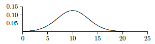
Figure \(\PageIndex{3}\). Normal density function for the defective chips example.

Now how do we measure how unlikely it is that under normal circumstances we would see \(15\) defective chips? We can't compute the probability of exactly \(15\) defective chips, as this would be \(\displaystyle\int_{15}^{15} f(x)\,dx = 0\). We could compute \(\displaystyle\int_{14.5}^{15.5} f(x)\,dx \approx 0.036\); this means there is only a \(3.6\%\) chance that the number of defective chips is \(15\). (We cannot compute these integrals exactly; computer software has been used to approximate the integral values in this discussion.) But this is misleading: even for the "most likely" outcome \(\displaystyle\int_{9.5}^{10.5} f(x)\,dx \approx 0.126\), which although it is larger, it is still small. The most useful question, in most circumstances, is this: how likely is it that the number of defective chips is "far from" the mean? For example, how likely, or unlikely, is it that the number of defective chips is different by \(5\) or more from the expected value of \(10\)? This is the probability that the number of defective chips is less than \(5\) or larger than \(15\), namely \[\int_{-\infty}^{5} f(x)\,dx + \int_{15}^{\infty} f(x)\,dx \approx 0.11.\nonumber\] So there is an \(11\%\) chance that this happens---not large, but not tiny. Hence the \(15\) defective chips does not appear to be cause for alarm: about one time in nine we would expect to see the number of defective chips \(5\) or more away from the expected \(10\). How about if there were \(20\) defective? Here we compute \[\int_{-\infty}^{0} f(x)\,dx + \int_{20}^{\infty} f(x)\,dx \approx 0.0015.\nonumber\] So there is only a \(0.15\%\) chance that the number of defective chips is \(10\) or more away from the mean; this would typically be interpreted as being too suspicious to ignore---it shouldn't happen if the process is running normally.

The big question, of course, is what level of improbability should trigger concern? That depends to some degree on the application, and in particular on the consequences of getting it wrong in one direction or the other. If we're wrong, do we lose a little money? A lot of money? Do people die? In general, the standard choices are \(5\%\) and \(1\%\). So what we should do is find the number of defective chips that has only, let us say, a \(1\%\) chance of occurring under normal circumstances, and use that as the relevant number. In other words, we want to know when \[\int_{-\infty}^{10-r} f(x)\,dx + \int_{10+r}^{\infty} f(x)\,dx \lt 0.01.\nonumber\] A bit of trial and error shows that with \(r=8\) the value is about \(0.011\), and with \(r=9\) it is about \(0.004\), so if the number of defective chips is \(19\) or more, or \(1\) or fewer, we should look for problems. If the number is high, we worry that the manufacturing process has a problem, or conceivably that the process that tests for defective chips is not working correctly and is flagging good chips as defective. If the number is too low, we suspect that the testing procedure is broken, and is not detecting defective chips.

Exercises \(\PageIndex{}\)

Exercise \(\PageIndex{1}\)

Verify that \(\displaystyle\int_1^\infty e^{-x/2}\,dx=2/\sqrt{e}\).

Exercise \(\PageIndex{2}\)

Show that the function in example \(\PageIndex{5}\) is a probability density function. Compute the mean and standard deviation.

Answer

\(\mu=\sigma=\dfrac{1}{c}.\)

Exercise \(\PageIndex{3}\)

Compute the mean and standard deviation of the uniform distribution on \([a,b]\). (See example \(\PageIndex{3}\).)

Answer

\(\mu=\dfrac{b+a}{2},\quad\sigma=\dfrac{b-a}{2\sqrt{3}}.\)

Exercise \(\PageIndex{4}\)

What is the expected value of one roll of a fair six-sided die?

Answer

\(7/2\).

Exercise \(\PageIndex{5}\)

What is the expected sum of one roll of three fair six-sided dice?

Answer

\(21/2\).

Exercise \(\PageIndex{6}\)

Let \(\mu\) and \(\sigma\) be real numbers with \(\sigma\gt 0\). Show that \[N(x) = \dfrac{1}{\sqrt{2\pi}\sigma}exp\left(-{(x-\mu)^2\over 2\sigma^2}\right)\nonumber\] is a probability density function. You will not be able to compute this integral directly; use a substitution to convert the integral into the one from example \(\PageIndex{4}\). The function \(N\) is the probability density function of a normal distribution. Show that the mean of this normal distribution is \(\mu\) and that the standard deviation is \(\sigma\).

Exercise \(\PageIndex{7}\)

Let \[\displaystyle f(x) = \cases{\displaystyle{1\over x^2 } & $x \ge 1,$\cr 0 & $x < 1.$\cr}\nonumber\] Show that \(f\) is a probability density function, and that the distribution has no mean.

Exercise \(\PageIndex{8}\)

Let \(f(x) = \cases{ x & $-1\le x \le 1,$\cr 1 & $1 \lt x \le 2,$\cr 0 & otherwise.\cr}\) Show that \(\displaystyle\int_{-\infty }^\infty f(x)\,dx = 1.\quad\) Is \(f\) a probability density function? Justify your answer.

Answer

No, because \(f(x) \lt 0\) for \(-1 \le x \lt 0.\)

Exercise \(\PageIndex{9}\)

If you have access to appropriate software, find \(r\) so that \(\displaystyle\int_{-\infty}^{10-r} f(x)\,dx + \int_{10+r}^{\infty} f(x)\,dx \approx0.05.\) Discuss the impact of using this new value of \(r\) to decide whether to investigate the chip manufacturing process.

Answer

\(r=6.\)

Contributors and Attributions

• David Guichard (Whitman College)

• Integrated by Justin Marshall.