1.6: Predator Response

Interactions of predators and prey are often studied in ecology. Professor C.S. ("Buzz") Holling, (a former Director of the Institute of Animal Resource Ecology at the University of British Columbia) described three types of predators, termed "Type I", "Type II" and "Type III", according to their ability to consume prey as the prey density increases. The three Holling "predator functional responses" are shown in Figure 1.10.

Figure 1.10: Holling’s Type I, II, and III predator response. The predation rate \(P(x)\) is the number of prey eaten by a predator per unit time. Note that the predation rate depends on the prey density \(x\).

Quick Concept Checks

Match the predator responses shown in Figure \(1.10\) with the descriptions given below

1. As a predator, I get satiated and cannot keep eating more and more prey.
2. I can hardly find the prey when the prey density is low, but I also get satiated at high prey density.
3. The more prey there is, the more I can eat.

Hint: One of the curves “looks like a straight line" (so which function here is linear?). One of the choices is a power function. (Will it fit any of the other curves? why or why not?). Now consider the saturating curves and use our description of rational functions in Section 1.5 to select appropriate formulae for these functions.

Based on Figure 1.10, match the predator responses to functions shown below.

\[\begin{aligned} & P_{1}(x)=k x, \\ & P_{2}(x)=K \frac{x}{a+x}, \\ & P_{3}(x)=K x^{n}, \quad n \geq 2 \\ & P_{4}(x)=K \frac{x^{n}}{a^{n}+x^{n}}, \quad n \geq 2 \end{aligned} \nonumber \]

The generality of mathematics allows us to adapt concepts we studied in one setting (enzyme biochemistry) to an apparently new topic (behavior of predators).

A ladybug eating aphids

Here we use ideas developed so far to address a problem in population growth and biological control.

See this short video explanation of the ladybug Type III predator response to its aphid prey.

Featured Problem 1.3 (A balance of predation and aphid population growth)

Ladybugs are predators that love to eat aphids (their prey). Figure \(1.11\) provides data \(^{1}\) that supports the idea that ladybugs are type 3 predators.

Figure 1.11: The predation rate of a ladybug depends on its aphid (prey) density.

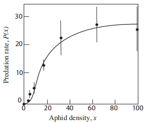
Let \(x=\) the number of aphids in some unit area (i.e., the density of the prey). Then the number of aphids eaten by a ladybug per unit time in that unit area will be called the predation rate and denoted \(P(x)\). The predation rate usually depends on the prey density, and we approximate that dependence by

\[P(x)=K \frac{x^{n}}{a^{n}+x^{n}}, \text { where } K, a>0 . \nonumber \]

Here we consider the case that \(n=2\). The aphids reproduce at a rate proportional to their number, so that the growth rate of the aphid population \(G\) (number of new aphids per hour) is

\[G(x)=r x \quad \text { where } \quad r>0 . \nonumber \]

1. For what aphid population density \(x\) does the predation rate exactly balance the aphid population growth rate?
2. Are there situations where the predation rate cannot match the growth rate? Explain your results in terms of the constants \(K, a, r\).

 

Hints and partial solution

(a) The wording "the predation rate exactly balances the reproduction rate" means that the two functions \(P(x)\) and \(G(x)\) are exactly equal. Hence, to solve this problem, equate \(P(x)=G(x)\) and determine the value of \(x\) (i.e., the number of aphids) at which this equality holds. You will find that one solution to this equation is \(x=0\). But if \(x \neq 0\), you can cancel one factor of \(x\) from both sides and rearrange the equation to obtain a quadratic equation whose solution can be written down (in terms of the positive constants \(K, r, a)\).

(b) The solution you find in (a) is only a real number (i.e. a real solution exists) if the discriminant (quantity inside the square-root) is positive. Determine when this situation can occur and interpret your answer in terms of the aphid and ladybugs.

Hint: Recall that a quadratic equation \(a x^2+b x+c=0\) has roots \(x=\frac{-b \pm \sqrt{b^2-4 a c}}{2 a}\). These roots are real provided \(b^2-4 a c \geq 0\).

The solution to this problem is based on solving a quadratic equation, and so, relies on the fact that we chose the value \(n=2\) in the predation rate. What happens if \(n>2\) ? How do we solve the same kind of problem if \(n=3,4\) etc? We return to this issue, and develop an approximate technique (Newton’s method) in a later chapter. \({ }^{1}\) MP Hassell, JH Lawton, and JR Beddington. Sigmoid functional responses by invertebrate predators and parasitoids. The Journal of Animal Ecology, 46(1):249-262, 1977

Use the sliders to manipulate the predation constants \(K, a\) and the aphid growth rate parameter \(r\). How many solutions are there to \(P(x)=G(x)\) ? Show that for some parameter values, there is only a trivial solution at \(x=0\). Make a connection between this observation and part (b) of Example 1.3.