1.8: Exercises

1.1. Power functions. Consider the power function

\[y=a x^{n}, \quad-\infty<x<\infty . \nonumber \]

Explain, possibly using a sketch, how the shape of the function changes when the coefficient \(a\) increases or decreases (for fixed \(n\) ). How is this change in shape different from the shape change that results from changing the power \(n\) ?

1.2. Transformations. Consider the graphs of the simple functions \(y=\) \(x, y=x^{2}\), and \(y=x^{3}\). Describe what happens to each of these graphs when the functions are transformed as follows: (a) \(y=A x, y=A x^{2}\), and \(y=A x^{3}\) where \(A>1\) is some constant. (b) \(y=x+a, y=x^{2}+a\), and \(y=x^{3}+a\) where \(a>0\) is some constant. (c) \(y=(x-b)^{2}\), and \(y=(x-b)^{3}\) where \(b>0\) is some constant.

1.3. Sketching transformations. Sketch the graphs of the following functions: (a) \(y=x^{2}\) (b) \(y=(x+4)^{2}\), (c) \(y=a(x-b)^{2}+c\) for the case \(a>0, b>0, c>0\). (d) Comment on the effects of the constants \(a, b, c\) on the properties of the graph of \(y=a(x-b)^{2}+c\).

1.4. Sketching polynomials. Use arguments from Section \(1.4\) to sketch graphs of the following polynomials: (a) \(y=2 x^{5}-3 x^{2}\), (b) \(y=x^{3}-4 x^{5}\).

1.5. Finding points of intersection.

(a) Consider the two functions \(f(x)=3 x^{2}\) and \(g(x)=2 x^{5}\). Find all points of intersection of these functions.

(b) Repeat for functions \(f(x)=x^{3}\) and \(g(x)=4 x^{5}\).

Note: finding these points of intersection is equivalent to calculating the zeros of the functions in Exercise 4.

1.6. Qualitative sketching skills.

(a) Sketch the graph of the function \(y=\rho x-x^{5}\) for positive and negative values of the constant \(\rho\). Comment on behavior close to zero and far away from zero.

(b) What are the zeros of this function and how does this depend on \(\rho\) ? (c) For what values of \(\rho\) would you expect that this function would have a local maximum ("peak") and a local minimum ("valley")?

1.7. Finding points of intersection. Consider functions \(f(x)=A x^{n}\) and \(g(x)=B x^{m}\). Suppose \(m>n>1\) are integers, and \(A, B>0\). Determine the values of \(x\) at which the the functions are the same - i.e. they intersect. Are there two places of intersection or three? How does this depend on the integer \(m-n\) ?

Note: The point \((0,0)\) is always an intersection point. Thus, we are asking: when is there only one more and when there are two more intersection points? See Exercise 5 for an example of both types.

1.8. More intersection points. Find the intersection of each pair of functions. (a) \(y=\sqrt{x}, y=x^{2}\) (b) \(y=-\sqrt{x}, y=x^{2}\) (c) \(y=x^{2}-1, \frac{x^{2}}{4}+y^{2}=1\).

1.9. Crossing the \(x\)-axis. Answer the following by solving for \(x\) in each case. Find all values of \(x\) for which the following functions cross the \(x\)-axis (equivalently: the zeros of the function, or roots of the equation \(f(x)=0\). (a) \(f(x)=I-\gamma x\), where \(I, \gamma\) are positive constants. (b) \(f(x)=I-\gamma x+\varepsilon x^{2}\), where \(I, \gamma, \varepsilon\) are positive constants. Are there cases where this function does not cross the \(x\) axis? (c) In the case where the root(s) exist in part (b), are they positive, negative or of mixed signs?

1.10. Crossing the \(x\)-axis. Answer Exercise 9 by sketching a rough graph of each of the functions in parts (a-b) and using these sketches to determine how many real roots there are and where they are located (positive vs. negative \(x\)-axis).

Note: this exercise provides qualitative analysis skills that are helpful in later applications.

1.11. Power functions. Consider the functions \(y=x^{n}, y=x^{1 / n}, y=x^{-n}\), where \(n\) is an integer \(n=1,2, \ldots)\).

(a) Which of these functions increases most steeply for values of \(x\) greater than 1?

(b) Which decreases for large values of \(x\) ?

(c) Which functions are not defined for negative \(x\) values?

(d) Compare the values of these functions for \(0<x<1\).

(e) Which of these functions are not defined at \(x=0\) ?

1.12. Roots of a quadratic. Find the range \(m\) such that the equation \(x^{2}-\) \(2 x-m=0\) has two unequal roots.

1.13. Rational Functions. Describe the shape of the graph of the function \(y=A x^{n} /\left(b+x^{m}\right)\) in two cases: (a) \(n>m\) and (b) \(m>n\).

1.14. Power functions with negative powers. Consider the function

\[f(x)=\frac{A}{x^{a}} \nonumber \]

where \(A>0, a>1\), with \(a\) an integer. This is the same as the function \(f(x)=A x^{-a}\), which is a power function with a negative power. (a) Sketch a rough graph of this function for \(x>0\). (b) How does the function change if \(A\) is increased? (c) How does the function change if \(a\) is increased?

1.15. Intersections of functions with negative powers. Consider two functions of the form

\[f(x)=\frac{A}{x^{a}}, \quad g(x)=\frac{B}{x^{b}} . \nonumber \]

Suppose that \(A, B>0, a, b>1\) and that \(A>B\). Determine where these functions intersect for positive \(x\) values.

1.16. Zeros of polynomials. Find all real zeros of the following polynomials: (a) \(x^{3}-2 x^{2}-3 x\), (b) \(x^{5}-1\), (c) \(3 x^{2}+5 x-2\). (d) Find the points of intersection of the functions \(y=x^{3}+x^{2}-2 x+1\) and \(y=x^{3}\).

1.17. Inverse functions. The functions \(y=x^{3}\) and \(y=x^{1 / 3}\) are inverse functions (see Section \(10.3\) for a discussion of inverse functions).

(a) Sketch both functions on the same graph for \(-2<x<2\) showing clearly where they intersect.

(b) The tangent line to the curve \(y=x^{3}\) at the point \((1,1)\) has slope \(m=\) 3 , whereas the tangent line to \(y=x^{1 / 3}\) at the point \((1,1)\) has slope \(m=1 / 3\). Explain the relationship of the two slopes.

1.18. Properties of a cube. The volume \(V\) and surface area \(S\) of a cube whose sides have length \(a\) are given by the formulae

\[V=a^{3}, \quad S=6 a^{2} . \nonumber \]

Note that these relationships are expressed in terms of power functions. The independent variable is \(a\), not \(x\). We say that " \(V\) is a function of \(a\) " (and also " \(S\) is a function of \(a\) ").

(a) Sketch \(V\) as a function of \(a\) and \(S\) as a function of \(a\) on the same set of axes. Which one grows faster as \(a\) increases?

(b) What is the ratio of the volume to the surface area; that is, what is \(\frac{V}{S}\) in terms of \(a\) ? Sketch a graph of \(\frac{V}{S}\) as a function of \(a\).

(c) The formulae above tell us the volume and the area of a cube of a given side length. Suppose we are given either the volume or the surface area and asked to find the side.

(i) Find the length of the side as a function of the volume (i.e. express \(a\) in terms of \(V\) ).

(ii) Find the side as a function of the surface area.

(iii) Use your results to find the side of a cubic tank whose volume is 1 litre.

(iv) Find the side of a cubic tank whose surface area is \(10 \mathrm{~cm}^{2}\).

Units. Note that 1 litre \(=10^{3} \mathrm{~cm}^{3}\).

1.19. Properties of a sphere. The volume \(V\) and surface area \(S\) of a sphere of radius \(r\) are given by the formulae

\[V=\frac{4 \pi}{3} r^{3}, \quad S=4 \pi r^{2} . \nonumber \]

Note that these relationships are expressed in terms of power functions with constant multiples such as \(4 \pi\). The independent variable is \(r\), not \(x\). We say that " \(V\) is a function of \(r\) " (and also " \(S\) is a function of \(r\) ").

(a) Sketch \(V\) as a function of \(r\) and \(S\) as a function of \(r\) on the same set of axes. Which one grows faster as \(r\) increases?

(b) What is the ratio of the volume to the surface area; that is, what is \(\frac{V}{S}\) in terms of \(r\) ? Sketch a graph of \(\frac{V}{S}\) as a function of \(r\).

(c) The formulae above tell us the volume and the area of a sphere of a given radius. But suppose we are given either the volume or the surface area and asked to find the radius.

(i) Find the radius as a function of the volume (i.e. express \(r\) in terms of \(V\) ).

(i) Find the radius as a function of the surface area.

(i) Use your results to find the radius of a balloon whose volume is 1 litre.

(i) Find the radius of a balloon whose surface area is \(10 \mathrm{~cm}^{2}\)

1.20. The size of cell. Consider a cell in the shape of a thin cylinder (length \(L\) and radius \(r\) ). Assume that the cell absorbs nutrient through its surface at rate \(k_{1} S\) and consumes nutrients at rate \(k_{2} V\) where \(S, V\) are the surface area and volume of the cylinder. Here we assume that \(k_{1}=12 \mu \mathrm{M} \mu \mathrm{m}^{-2}\) per min and \(k_{2}=2 \mu \mathrm{M} \mu \mathrm{m}^{-3}\) per min.

Units. Note that \(\mu \mathrm{M}\) is \(10^{-6}\) moles and \(\mu \mathrm{m}\) is \(10^{-6}\) meters.

(a) Use the fact that a cylinder (without end-caps) has surface area \(S=\) \(2 \pi r L\) and volume \(V=\pi r^{2} L\) to determine the cell radius such that the rate of consumption exactly balances the rate of absorption.

(b) What do you expect happens to cells with a bigger or smaller radius?

(c) How does the length of the cylinder affect this nutrient balance?

1.21. Energy equilibrium for Earth. This exercise focuses on Earth’s temperature, climate change, and sustainability.

(a) Complete the calculation for Example \(1.5\) by solving for the temperature \(T\) of the Earth at which incoming and outgoing radiation energies balance.

(b) Assume that greenhouse gases decrease the emissivity \(\varepsilon\) of the Earth’s atmosphere. Explain how this would affect the Earth’s temperature.

(c) Explain how the size of the Earth affects its energy balance according to the model.

(d) Explain how the albedo \(a\) affects the Earth’s temperature.

1.22. Allometric relationship. Properties of animals are often related to their physical size or mass. For example, the metabolic rate of the animal \((R)\), and its pulse rate \((P)\) may be related to its body mass \(m\) by the approximate formulae \(R=A m^{b}\) and \(P=C m^{d}\), where \(A, C, b, d\) are positive constants. Such relationships are known as allometric relationships.

(a) Use these formulae to derive a relationship between the metabolic rate and the pulse rate (hint: eliminate \(m\) ).

(b) A similar process can be used to relate the Volume \(V=(4 / 3) \pi r^{3}\) and surface area \(S=4 \pi r^{2}\) of a sphere to one another. Eliminate \(r\) to find the corresponding relationship between volume and surface area for a sphere.

1.23. Rate of a very simple chemical reaction. We consider a chemical reaction that does not saturate, and a simple linear relationship between reaction speed and reactant concentration.

A chemical is being added to a mixture and is used up in a reaction. The rate of change of the chemical, (also called "the rate of the reaction") \(v \mathrm{M} / \mathrm{sec}\) is observed to follow a relationship

Units. Note that M stands for Molar, which is the number of moles per litre.

\[v=a-b c \nonumber \]

where \(c\) is the reactant concentration (in units of \(\mathbf{M}\) ) and \(a, b\) are positive constants.

Note: \(v\) is considered to be a function of \(c\), and moreover, the relationship between \(v\) and \(c\) is assumed to be linear.

Figure 1.12: Figure for Exercise 23; rate of a chemical reaction. Assume that the intercept of the line on the \(c\) axis is at \(0.01 \mathrm{M}\)

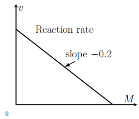
(a) What units should \(a\) and \(b\) have to make this equation consistent? Note: in an equation such as \(v=a-b c\), each of the three terms must have the same units. Otherwise, the equation would not make sense.

(b) Use the information in the graph shown in Figure \(1.12\) (and assume that the intercept on the \(c\) axis is at \(0.01 \mathrm{M})\) to find the values of \(a\) and \(b\) (hint: find the equation of the line in the figure, and compare it to the relationship \(v=a-b c)\).

(c) What is the rate of the reaction when \(c=0.005 \mathrm{M}\) ?

1.24. Michaelis-Menten kinetics. Consider the Michaelis-Menten kinetics where the speed of an enzyme-catalyzed reaction is given by \(v=\) \(K x /\left(k_{n}+x\right)\)

(a) Explain the statement that "when \(x\) is large there is a horizontal asymptote" and find the value of \(v\) to which that asymptote approaches.

(b) Determine the reaction speed when \(x=k_{n}\) and explain why the constant \(k_{n}\) is sometimes called the "half-max" concentration.

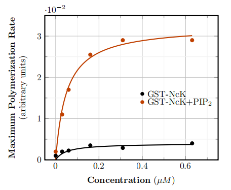
1.25. A polymerization reaction. Consider the speed of a polymerization reaction shown in Figure 1.13. Here the rate of the reaction is plotted as a function of the substrate concentration; this experiment concerned the polymerization of actin, an important structural component of cells; data from [Rohatgi et al., 2001]. The experimental points are shown as dots, and a Michaelis-Menten curve has been drawn to best fit these points. Use the data in the figure to determine approximate values of \(K\) and \(k_{n}\) in the two treatments shown.

Figure 1.13: Figure for Exercise. 25; speed of polymerization. another. Consider the Hill functions

1.26. Hill functions. Hill functions are sometimes used to represent a biochemical "switch," that is a rapid transition from one state to

\[y_{1}=\frac{x^{2}}{1+x^{2}}, \quad y_{2}=\frac{x^{5}}{1+x^{5}}, \nonumber \]

(a) Where do these functions intersect?

(b) What are the asymptotes of these functions?

(c) Which of these functions increases fastest near the origin?

(d) Which is the sharpest "switch" and why?

1.27. Transforming a Hill function to a linear relationship. A Hill function is a nonlinear function - but if we redefine variables, we can transform it into a linear relationship. The process is analogous to transforming Michaelis-Menten kinetics into a Lineweaver-Burk plot, as discussed in Appendix G.1.

(a) Determine how to define appropriate variables \(X\) and \(Y\) (in terms of the original variables \(x\) and \(y\) ) so that the Hill function \(y=\) \(A x^{3} /\left(a^{3}+x^{3}\right)\) is turned into a linear relationship between \(X\) and \(Y\).

(b) Indicate how the slope and intercept of the line are related to the original constants \(A, a\) in the Hill function.

1.28. Hill function and sigmoidal chemical kinetics. It is known that the rate \(v\) at which a certain chemical reaction proceeds depends on the concentration of the reactant \(c\) according to the formula

\[v=\frac{K c^{2}}{a^{2}+c^{2}} \nonumber \]

where \(K, a\) are some constants. When the chemist plots the values of the quantity \(1 / v\) (on the " \(y\) " axis) versus the values of \(1 / c^{2}\) (on the " \(x\) axis"), she finds that the points are best described by a straight line with \(y\)-intercept 2 and slope 8 . Use this result to find the values of the constants \(K\) and \(a\).

1.29. Lineweaver-Burk plots. Shown in the Figure 1.14(a) and (b) are two Lineweaver-Burk plots (see Appendix G.1). By noting properties of these figures comment on the comparison between the following two enzymes:

(a) Enzyme (1) and (2).

(b) Enzyme (1) and (3).

1.30. Michaelis-Menten enzyme kinetics. The rate of an enzymatic reaction according to the Michaelis-Menten kinetics assumption is

\[v=\frac{K c}{k_{n}+c}, \nonumber \]

where \(c\) is concentration of substrate (shown on the \(x\)-axis) and \(v\) is the reaction speed (given on the \(y\)-axis). Consider the data points given in Table 1.2.

Figure 1.14: Figure for Exercise 29: Lineweaver-Burk plots.

Substrate concentration	\(\mathrm{nM}\)	\(c\)	5	10	20	40	50	100
Reaction speed	\(\mathrm{nM} / \mathrm{min}\)	\(v\)	\(0.068\)	\(0.126\)	\(0.218\)	\(0.345\)	\(0.39\)	\(0.529\)

Table 1.2: Chemical reaction speed data.

(a) Convert this data to a Lineweaver-Burk (linear) relationship (see Appendix G.1 for discussion).

(b) Plot the transformed data values on a graph or spreadsheet, and estimate the slope and \(y\)-intercept of the line you get.

(c) Use these results to find the best estimates for \(K\) and \(k_{n}\).

1.31. Spacing in a school of fish. According to the biologist Breder [Breder, 1951], two fish in a school prefer to stay some specific distance apart. Breder suggested that the fish that are a distance \(x\) apart are attracted to one another by a force \(F_{A}(x)=A / x^{a}\) and repelled by a second force \(F_{R}(x)=R / x^{r}\), to keep from getting too close. He found the preferred spacing distance (also called the individual distance) by determining the value of \(x\) at which the repulsion and the attraction exactly balance.

Find the individual distance in terms of the quantities \(A, R, a, r\) (all assumed to be positive constants.)