10.2: Derivatives of Exponential Functions

Learning Objectives

1. Using the definition of the derivative, calculate the derivative of the function \(y=a^{x}\) for an arbitrary base \(a>0\).
2. Describe the significance of the special base \(e\).
3. Summarize the properties of the function \(e^{x}\), its derivatives, and how to manipulate it algebraically.
4. Recall the fact that the function \(y=e^{k x}\) has a derivative that is proportional to the same function \(\left(y=e^{k x}\right)\).

A screencast with the calculations for this section and motivation for the natural base \(e\). Edu.Cr.

Calculating the derivative of \(a^{x}\)

In this section we show how to compute the derivative of the exponential function. Rather then restricting attention to the special case \(y=2^{x}\), we consider an arbitrary positive constant \(a\) as the base. Note that the base has to be positive to ensure that the function is defined for all real \(x\). For \(a>0\) let

\[y=f(x)=a^{x} \nonumber \]

Then, using the definition of the derivative,

\[\begin{aligned} \frac{d a^{x}}{d x} & =\lim _{h \rightarrow 0} \frac{\left(a^{x+h}-a^{x}\right)}{h} \\ & =\lim _{h \rightarrow 0} \frac{\left(a^{x} a^{h}-a^{x}\right)}{h} \\ & =\lim _{h \rightarrow 0} a^{x} \frac{\left(a^{h}-1\right)}{h} \\ & =a^{x}\left[\lim _{h \rightarrow 0} \frac{a^{h}-1}{h}\right] \end{aligned} \nonumber \]

The variable \(x\) appears only in the common factor \(a^{x}\) that can be factored out. The limit applies to \(h, \operatorname{not} x\). The terms inside square brackets depend only on the base \(a\) and on \(h\), but once the limit is evaluated, that term is some constant (independent of \(x\) ) that we denote by \(C_{a}\). To summarize, we have found that

The derivative of an exponential function \(a^{x}\) is of the form \(C_{a} a^{x}\) where \(C_{a}\) is a constant that depends only on the base \(a\).

We now examine this in more detail with bases 2 and 10.

Mastered Material Check

10. Describe geometrically the derivative of \(a^{x}\).

Example 10.3 (Derivative of \(2^{x}\) )

Write down the derivative of \(y=2^{x}\) using the above result.

Solution

For base \(a=2\), we have

\[\frac{d 2^{x}}{d x}=C_{2} \cdot 2^{x} \nonumber \]

where

\[C_{2}(h)=\lim _{h \rightarrow 0} \frac{2^{h}-1}{h} \approx \frac{2^{h}-1}{h} \text { for small } h . \nonumber \]

The decimal expansion value of \(C_{2}\) is determined in the next example.

Example 10.4 (The value of \(C_{2}\) )

Find an approximation for the value of the constant \(C_{2}\) in Example \(10.3\) by calculating the value of the ratio \(\left(2^{h}-1\right) / h\) for small (finite) values of \(h\), e.g., \(h=0.1,0.01\), etc. Do these successive approximations for \(C_{2}\) value approach a fixed real number?

Solution

We take these successively smaller values of \(h\) and compute the value of \(C_{2}=\left(2^{h}-1\right) / h\) on a spreadsheet.

The results are shown in Table \(10.1\), where we find that \(C_{2} \approx 0.6931\). (The actual value has an infinitely long decimal expansion that we here represent by its first few digits.) Thus, the derivative of \(2^{x}\) is

\[\frac{d 2^{x}}{d x}=C_{2} \cdot 2^{x} \approx(0.6931) \cdot 2^{x} . \nonumber \]

Table 10.1: The constant \(C_{2}\) in Example \(10.4\) is found by letting \(h\) get smaller and smaller. The value converges to \(C_{2}=0.693147\) Example \(10.5\) (The base 10 and the derivative of \(10^{x}\) ) Determine the derivative of \(y=f(x)=10^{x}\).

\(\boldsymbol{h}\)	\(\boldsymbol{C}_{2}\)
\(\cdots 0.1\)	\(0.717735\)
\(0.01\)	\(0.695555\)
\(0.001\)	\(0.693387\)
\(0.0001\)	\(0.693171\)
\(0.00001\)	\(0.693150\)
\(0.000001\)	\(0.693147\)
\(0.0000001\)	\(0.693147\)

Link to Google Sheets. The constant \(C_{a}\) in the derivative of \(a^{x}\) is calculated on this spreadsheet for \(a=2\). You can copy and paste this to our own spreadsheet and experiment with the value of the base \(a\). Try to find a value of \(a\) between 2 and 3 for which \(C_{a}\) is close to 1.0.

Example 10.5 (The base 10 and the derivative of \(10^x\) )

Determine the derivative of \(y=f(x)=10^x\)

Solution

For base 10 we have

\[C_{10}(h) \approx \frac{10^{h}-1}{h} \text { for small } h . \nonumber \]

We find, by similar approximation (Table 10.2), that \(C_{10} \approx 2.3026\), so that

\[\frac{d 10^{x}}{d x}=C_{10} \cdot 10^{x} \approx(2.3026) \cdot 10^{x} . \nonumber \]

Thus, the derivative of \(y=a^{x}\) is proportional to itself, but the constant of proportionality \(\left(C_{a}\right)\) depends on the base.

Table 10.2: As in Table \(10.1\) but for the constant \(C_{10}\) in Example 10.5. (The advantage of using a spreadsheet is that we only need to change one cell to obtain this new set of values.)

\(h\)	\(C_{10}\)
\(0.1\)	\(2.589254\)
\(0.01\)	\(2.329299\)
\(0.001\)	\(2.305238\)
\(0.0001\)	\(2.302850\)
\(0.00001\)	\(2.302612\)
\(0.000001\)	\(2.302588\)
\(0.0000001\)	\(2.302585\)

Mastered Material Check

11. What does it mean for a function \(f(x)\) to be proportional to itself?

The natural base \(e\) is convenient for calculus

In Examples 10.3-10.5, we found that the derivative of \(a^{x}\) is \(C_{a} a^{x}\), where the constant \(C_{a}\) depends on the base. These constants are somewhat inconvenient, but unavoidable if we use an arbitrary base. Here we ask:

Does there exists a convenient base (to be called " \(e\) ") for which the constant is particularly simple, namely such that \(C_{e}=1\) ?

This is the property of the natural base that we next identify.

We can determine such a hypothetical base using only the property that

\[C_{e}=\lim _{h \rightarrow 0} \frac{e^{h}-1}{h}=1 . \nonumber \]

This means that for small \(h\)

\[\frac{e^{h}-1}{h} \approx 1, \nonumber \]

so that

\[e^{h}-1 \approx h \Rightarrow e^{h} \approx h+1 \Rightarrow e \approx(1+h)^{1 / h} . \nonumber \]

More formally,

\[e=\lim _{h \rightarrow 0}(1+h)^{1 / h} \]

We can find an approximate decimal expansion for \(e\) by calculating the ratio in Equation (10.2.1) for some very small (but finite value) of \(h\) on a spreadsheet. Results are shown in Table 10.3.

Link to Google Sheets. The calculation of a decimal approximation to base \(e\) as shown in Table \(10.3\).

Table 10.3: We can use a spreadsheet to find a decimal approximation to the natural base \(e\) using Equation (10.1) and letting \(h\) approach zero.

\(\boldsymbol{h}\)	approximation to \(\boldsymbol{e}\)
\(0.1\)	\(2.5937425\)
\(0.01\)	\(2.7048138\)
\(0.001\)	\(2.7169239\)
\(0.0001\)	\(2.7181459\)
\(0.00001\)	\(2.7182682\)

We find (e.g. for \(h=0.00001\) ) that

\[e \approx(1.00001)^{100000} \approx 2.71826 . \nonumber \]

To summarize, we have found that for the special base, \(e\), we have the following property:

The derivative of the function \(e^{x}\) is \(e^{x}\).

The value of base \(e\) is obtained from the limit in Equation (10.2.1). This can be written in either of two equivalent forms.

The base of the natural exponential function is the real number defined as follows:

\[e=\lim _{h \rightarrow 0}(1+h)^{1 / h}=\lim _{n \rightarrow \infty}\left(1+\frac{1}{n}\right)^{n} . \nonumber \]

Mastered Material Check

12. Why can’t we simply plug in \(h=0\) into Equation (10.2.1) evaluate the limit?
13. Let \(h=\frac{1}{n}\) and rewrite Eqn (10.1).
14. Explain why each of Properties \(1 . \rightarrow 8\). hold for the function \(e^{x}\).

Properties of the function \(e^{x}\)

We list below some of the key features of the function \(y=e^{x}\). Note that all stem from basic manipulations of exponents as reviewed in Appendix B.1.

1. \(e^{a} e^{b}=e^{a+b}\) as with all similar exponent manipulations.
2. \(\left(e^{a}\right)^{b}=e^{a b}\) also stems from simple rules for manipulating exponents.
3. \(e^{x}\) is a function that is defined, continuous, and differentiable for all real numbers \(x\).
4. \(e^{x}>0\) for all values of \(x\).
5. \(e^{0}=1\), and \(e^{1}=e\).
6. \(e^{x} \rightarrow 0\) for increasing negative values of \(x\).
7. \(e^{x} \rightarrow \infty\) for increasing positive values of \(x\).
8. The derivative of \(e^{x}\) is \(e^{x}\) (shown in this chapter).

Use the slider to adjust the value of the base a in the function \(y=a^x\) ; Compare your result with the function \(y = e^x\). Explain what you see for \(a > 1\), \(a = 1\), \(0 < a < 1\) and \(a = 0\).

Example 10.6

1. Find the derivative of \(e^{x}\) at \(x=0\).
2. Show that the tangent line at that point is the line \(y=x+1\).

Solution

a) The derivative of \(e^{x}\) is \(e^{x}\). At \(x=0, e^{0}=1\).

b) The slope of the tangent line at \(x=0\) is therefore 1 . The tangent line goes through \(\left(0, e^{0}\right)=(0,1)\) so it has a \(y\)-intercept of 1 . Thus the tangent line at \(x=0\) with slope 1 is \(y=x+1\). This is shown in Figure 10.4.

Figure 10.4: The function \(y=e^{x}\) has the property that its tangent line at \(x=0\) has slope 1.

Review: On this graph of \(f(x)=e^{x}\) add a generic tangent line at any point \(x_{0}\). (See Sections 5.1-5.2). Adjust a slider for \(x_{0}\) to get the configuration shown in Figure 10.4. \(y\)

Composite derivatives involving exponentials

Using the derivative of \(e^{x}\) and the chain rule, we can now differentiate composite functions in which the exponential function appears.

Example 10.7

Find the derivative of \(y=e^{k x}\).

Solution

Letting \(u=k x\) gives \(y=e^{u}\). Applying the simple chain rule leads to,

\[\frac{d y}{d x}=\frac{d y}{d u} \frac{d u}{d x} \nonumber \]

but

\[\frac{d u}{d x}=k \quad \text { so } \quad \frac{d y}{d x}=e^{u} k=k e^{k x} . \nonumber \]

We highlight this result for future use:

The derivative of \(y=e^{k x}\) is

\[\frac{d y}{d x}=k e^{k x} . \nonumber \]

Example 10.8 (Chemical reactions)

According to the collision theory of bimolecular gas reactions, a reaction between two molecules occurs when the molecules collide with energy greater than some activation energy, \(E_{a}\), referred to as the Arrhenius activation energy. \(E_{a}>0\) is constant for the given substance. The fraction of bimolecular reactions in which this collision energy is achieved is

\[F=e^{-\left(E_{a} / R T\right)}, \nonumber \]

where \(T\) is temperature (in degrees Kelvin) and \(R>0\) is the gas constant. Suppose that the temperature \(T\) increases at some constant rate, \(C\), per unit time.

Determine the rate of change of the fraction \(F\) of collisions that result in a successful reaction.

Solution

This is a related rates problem involving an exponential function that depends on the temperature, which depends on time, \(F=e^{-\left(E_{a} / R T(t)\right)}\). We are asked to find the derivative of \(F\) with respect to time when the temperature increases.

We are given that \(d T / d t=C\). Let \(u=-E_{a} / R T\). Then \(F=e^{u}\). Using the chain rule,

\[\frac{d F}{d t}=\frac{d F}{d u} \frac{d u}{d T} \frac{d T}{d t} . \nonumber \]

Further, we have \(E_{a}, R, C\) are all constants, so

\[\frac{d F}{d u}=e^{u} \quad \text { and } \quad \frac{d u}{d T}=\frac{E_{a}}{R T^{2}} . \nonumber \]

Assembling these parts, we have

\[\frac{d F}{d t}=e^{u} \frac{E_{a}}{R T^{2}} C=C \frac{E_{a}}{R} T^{-2} e^{-\left(E_{a} / R T\right)}=\frac{C E_{a}}{R T^{2}} e^{-\left(E_{a} / R T\right)} . \nonumber \]

Thus, the rate of change of the fraction \(F\) of collisions that result in a successful reaction is given by the expression above.

Mastered Material Check

15. Let \(y=e^{5 x}\). What is \(\frac{d y}{d x}\) ?
16. Let \(y=e^{\pi x}\). What is \(\frac{d y}{d x}\) ?
17. List all constants in Example 10.8.
18. List all variables in Example 10.8.

Featured Problem \(10.1\) (Ricker model for fish population growth):

Salmon are fish with non-overlapping generations. The adults lay eggs that are fertilized by males before the entire population dies. The eggs hatch to form a new generation. In Featured Problem 1.1, we considered one model for fish populations. Here we discuss a second model, the Ricker Equation, wherein the fish population this year, \(N_{1}\), is related to the population last year, \(N_{0}\), by the rule

\[N_{1}=N_{0} e^{r\left(1-\frac{N_{0}}{K}\right)}, \quad r, K>0 \]

Here \(r\) is called an intrinsic growth rate, and \(K\) is the carrying capacity of the population.

Figure 10.5: The functional form of the Ricker equation.

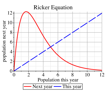
We investigate the following questions.

(a) Is there a population level \(N_{0}\) that would stay constant from one year to the next?

(b) Simplify the notation by setting \(x=N_{0}, y=N_{1}\). Compute the derivative \(d y / d x\) and interpret its meaning.

(c) What population level this year would result in the greatest possible population next year?

The function \(e^{x}\) satisfies a new kind of equation

We divert our attention momentarily to an interesting observation. We have seen that the function

\[y=f(x)=e^{x} \nonumber \]

satisfies the relationship

\[\frac{d y}{d x}=f^{\prime}(x)=f(x)=y . \nonumber \]

In other words, when differentiating, we get the same function back again. We summarize this observation:

The function \(y=f(x)=e^{x}\) is equal to its own derivative. It hence satisfies the equation

\[\frac{d y}{d x}=y . \nonumber \]

An equation linking a function and its derivative(s) is called a differential equation.

This is a new type of equation, unlike others previously seen in this course. In Chapters 11-13 we show that these differential equations have many applications to biology, physics, chemistry, and science in general.

Adjust the sliders to observe how the parameters \(K\) and \(r\) affect the Ricker equation 10.2.2. What is special about the intersection of the two curves shown?