11.2: Differential equation for unlimited population growth

Learning Objectives

1. Recall the derivation of a model for human population growth and describe how it leads to a differential equation.
2. Identify that the solution to that equation is an exponential function.
3. Define per capita birth rates and rates of mortality, and explain the process of estimating their values from assumptions about the population.
4. Compute the doubling time of a population from its growth rate and vice versa.

A screencast summary of the model for (unlimited) human population growth.

Differential equations are important because they turn up in the study of many natural processes that vary continuously. In this section we examine the way that a simple differential equation arises when we study continuous uncontrolled population growth.

Here we set up a mathematical model for population growth. Let \(N(t)\) be the number of individuals in a population at time \(t\). The population changes with time due to births and mortality. (Here we ignore migration). Consider the changes that take place in the population size between time \(t\) and \(t+h\), where \(\Delta t=h\) is a small time increment. Then

\[N(t+h)-N(t)=\left[\begin{array}{c} \text { Change } \\ \text { in } N \end{array}\right]=\left[\begin{array}{c} \text { Number of } \\ \text { births } \end{array}\right]-\left[\begin{array}{c} \text { Number of } \\ \text { deaths } \end{array}\right] \]

Equation (11.2.1) is just a "book-keeping" equation that keeps track of people entering and leaving the population. It is sometimes called a balance equation. We use it to derive a differential equation linking the derivative of \(N\) to the value of \(N\) at the given time.

Notice that dividing each term by the time interval \(h\), we obtain

\[\frac{N(t+h)-N(t)}{h}=\left[\frac{\text { Number of births }}{h}\right]-\left[\frac{\text { Number of deaths }}{h}\right] . \nonumber \]

The term on the left "looks familiar". If we shrink the time interval, \(h \rightarrow 0\), this term is a derivative \(d N / d t\), so

\[\frac{d N}{d t}=\left[\begin{array}{c} \text { Rate of } \\ \text { change of N } \\ \text { per unit time } \end{array}\right]=\left[\begin{array}{c} \text { Number of } \\ \text { births per } \\ \text { unit time } \end{array}\right]-\left[\begin{array}{c} \text { Number of } \\ \text { deaths per } \\ \text { unit time } \end{array}\right] \nonumber \]

For simplicity, we assume that all individuals are identical and that the number of births per unit time is proportional to the population size. Denote by \(r\) the constant of proportionality. Similarly, we assume that the number of deaths per unit time is proportional to population size with \(m\) the constant of proportionality.

Mastered Material Check

12. What is the dependent variable in this model? The independent variable?
13. What are the units associated with each variable in this model?
14. What does " \(x\) is proportional to \(y\) " mean?

Both \(r\) and \(m\) have meanings: \(r\) is the average per capita birth rate, and \(m\) is the average per capita mortality rate . Here, both are assumed to be fixed positive constants that carry units of \(1 /\) time. This is required to make the units match for every term in Equation (11.4). Then

\[\begin{gathered} r=\text { per capita birth rate }=\frac{\text { number births per unit time }}{\text { population size }}, \\ m=\text { per capita mortality rate }=\frac{\text { number deaths per unit time }}{\text { population size }} . \end{gathered} \nonumber \]

Consequently, we have

\[\begin{aligned} \text { Number of births per unit time } & =r N, \\ \text { Number of deaths per unit time } & =m N . \end{aligned} \nonumber \]

We refer to constants such as \(r, m\) as parameters. In general, for a given population, these would have specific numerical values that could be found through experiment, by collecting data, or by making simple assumptions. In Section 11.2, we show how some elementary assumptions about birth and mortality could help to estimate approximate values of \(r\) and \(m\).

Taking the assumptions and the form of the balance equation (11.2.1) together we have arrived at:

\[\frac{d N}{d t}=r N-m N=(r-m) N \]

This is a differential equation: it links the derivative of \(N(t)\) to the function \(N(t)\). By solving the equation (i.e. identifying its solution), we are be able to make a projection about how fast a population is growing.

Define the constant \(k=r-m\). Then \(k\) is the net growth rate, of the population, so

\[\frac{d N}{d t}=k N, \quad \text { for } k=(r-m) . \nonumber \]

Suppose we also know that at time \(t=0\), the population size is \(N_{0}\). Then:

• The function that describes population over time is (by previous results),

\[N(t)=N_{0} e^{k t}=N_{0} e^{(r-m) t} \]

(The result is identical to what we saw previously, but with \(N\) rather than \(y\) as the time-dependent function. We can easily check by differentiation that this function satisfies Equation (11.2.2).)

• Since \(N(t)\) represents a population size, it has to be non-negative to have biological relevance. This is true so long as \(N_{0} \geq 0\).
• The initial condition \(N(0)=N_{0}\), allows us to specify the (otherwise arbitrary) constant multiplying the exponential function.
• If \(k<0\), or equivalently, \(r<m\) then more people die on average than are born, so that the population shrinks and (eventually) go extinct.

Mastered Material Check

15. If there are 10 births/year in a population of size 1000 , what is the birth rate \(r\) ? Give units.
16. If there are 11 deaths/year in a population of size 1000 , what is the mortality rate \(m\) ? Give units.
17. Given the above conditions, what is the net growth rate \(k\) for such a population? Give units. Is the population growing or shrinking? - The population grows provided \(k>0\) which happens when \(r-m>0\) i.e. when birth rate exceeds mortality rate.

A simple model for human population growth

The differential equation (11.2.2) and its initial condition led us to predict that a population grows or decays exponentially in time, according to Equation (11.2.3). We can make this prediction quantitative by estimating the values of parameters \(r\) and \(m\). To this end, let us consider the example of a human population and make further simplifying assumptions. We measure time in years.

Assumptions.

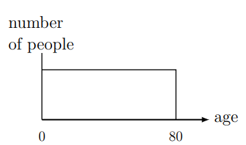
• The age distribution of the population is "flat", i.e. there are as many 10 year-olds as 70 year olds. Of course, this is quite inaccurate, but a good place to start since it is easy to estimate some of the quantities we need. Figure \(11.2\) shows such a uniform age distribution.

Figure 11.2: We assume a uniform age distribution to to determine the fraction of people who are fertile (and can give birth) or who are old (and likely to die). While slightly silly, this simplification helps estimate the desired parameters.

• The sex ratio is roughly \(50 \%\). This means that half of the population is female and half male.
• Women are fertile and can have babies only during part of their lives: we assume that the fertile years are between age 15 and age 55, as shown in Figure 11.3.

Figure 11.3: We assume that only women between the ages of 15 and 55 years old are fertile and can give birth. Then, according to our uniform age distribution assumption, half of all women are between these ages and hence fertile.

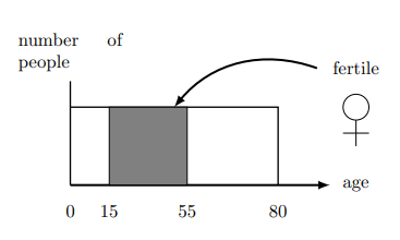
• A lifetime lasts 80 years. This means that for half of that time a given woman can contribute to the birth rate, or that \(\frac{(55-15)}{80}=50 \%\) of women alive at any time are able to give birth.
• During a woman’s fertile years, we assume that on average, she has one baby every 10 years.
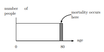
• We assume that deaths occur only from old age (i.e. we ignore disease, war, famine, and child mortality.)
• We assume that everyone lives precisely to age 80 , and then dies instantly.

Figure 11.4: We assume that the people in the age bracket 79-80 years old all die each year, and that those are the only deaths. This, too, is a silly assumption, but makes it easy to estimate mortality in the population.

Based on the above assumptions, we can estimate the birthrate parameter \(r\) as follows:

\[r=\frac{\text { number women }}{\text { population }} \cdot \frac{\text { years fertile }}{\text { years of life }} \cdot \frac{\text { number babies per woman }}{\text { number of years }} \nonumber \]

Thus we compute that

\[r=\frac{1}{2} \cdot \frac{1}{2} \cdot \frac{1}{10}=0.025 \text { births per person per year. } \nonumber \]

Note that this value is now a rate per person per year, averaged over the entire population (male and female, of all ages). We need such an average rate since our model of Equation (11.5) assumes that individuals "are identical". We now have an approximate value for the average human per capita birth rate, \(r \approx 0.025\) per year.

Next, using our assumptions, we estimate the mortality parameter, \(m\). With the flat age distribution shown in Figure 11.2, there would be a fraction of \(1 / 80\) of the population who are precisely removed by mortality every year (i.e. only those in their \(80^{\text {th }}\) year.) In this case, we can estimate that the per capita mortality is:

\[m=\frac{1}{80}=0.0125 \text { deaths per person per year. } \nonumber \]

The net per capita growth rate is \(k=r-m=0.025-0.0125=0.0125\) per person per year. We often refer to the constant \(k\) as a growth rate constant and we also say that the population grows at the rate of \(1.25 \%\) per year.

Example 11.3

Using the results of this section, find a prediction for the population size \(N(t)\) as a function of time \(t\).

Solution

We have found that our population satisfies the equation

\[\frac{d N}{d t}=(r-m) N=k N=0.0125 N, \nonumber \]

so that

\[N(t)=N_{0} e^{0.0125 t} \]

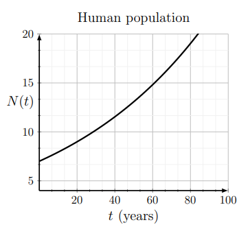
where \(N_{0}\) is the starting population size. Figure \(11.5\) illustrates how this function behaves, using a starting value of \(N(0)=N_{0}=7\) billion.

Figure 11.5: Projected world population (in billions) over 100 years, based on the model in Equation (11.2.4) and assuming that the initial population is \(\approx 7\) billion.

Mastered Material Check

18. Under these assumptions, for a population size of 800 , how many male 35 year-olds would you expect? Women in their 60’s?
19. Is the fertility assumption reasonable? Why or why not?
20. Explain the units attached to the birthrate parameter \(r\).

Example 11.4 (Human population in 100 years)

Given the initial condition \(N(0)=7\) billion, determine the size of the human population at \(t=100\) years predicted by the model.

Solution

At time \(t=0\), the population is \(N(0)=N_{0}=7\) billion. Then in billions,

\[N(t)=7 e^{0.0125 t} \nonumber \]

so that when \(t=100\) we would have

\[N(100)=7 e^{0.0125 \cdot 100}=7 e^{1.25}=7 \cdot 3.49=24.43 . \nonumber \]

Thus, with a starting population of 7 billion, there would be about \(24.4\) billion after 100 years based on the uncontrolled continuous growth model.

A critique. Before leaving our population model, we should remember that our projections hold only so long as some rather restrictive assumptions are made. We have made many simplifications, and ignored many features that would seriously affect these results. These include (among others),

• variations in birth and mortality rates that stem from competition for resources and,
• epidemics that take hold when crowding occurs, and
• uneven distributions of resources or space.

We have also assumed that the age distribution is uniform (flat), but that is not accurate: the population grows only by adding new infants, and this would skew the distribution even if it is initially uniform. All these factors suggest that some "healthy skepticism" should be applied to any model predictions. Predictions may cease to be valid if model assumptions are not satisfied. This caveat will lead us to think about more realistic models for population growth. Certainly, the uncontrolled exponential growth would not be sustainable in the long run. That said, such a model is a good starting point for a first description of population growth, later to be adjusted.

Mastered Material Check

21. Based on Figure 11.5, when would we expect the human population to reach 15 billion?

Growth and doubling

In Chapter 10, we used base 2 to launch our discussion of exponential growth and population doublings. We later discovered that base \(e\) is more convenient for calculus, having a more elegant derivative. We also saw in Chapter 10 , that bases of exponents can be inter-converted. These skills are helpful in our discussion of doubling times below.

The doubling time. How long would it take a population to double, given that it is growing exponentially with growth rate \(k\) ? We seek a time \(t\) such that \(N(t)=2 N_{0}\). Then

\[N(t)=2 N_{0} \quad \text { and } \quad N(t)=N_{0} e^{k t}, \nonumber \]

implies that the population has doubled when \(t\) satisfies

\[2 N_{0}=N_{0} e^{k t}, \quad \Rightarrow \quad 2=e^{k t} \Rightarrow \ln (2)=\ln \left(e^{k t}\right)=k t . \nonumber \]

We solve for \(t\). Thus, the doubling time, denoted \(\tau\) is:

\[\tau=\frac{\ln (2)}{k} . \nonumber \]

Example 11.5 (Human population doubling time)

Determine the doubling time for the human population based on the results of our approximate growth model.

Solution

We have found a growth rate of roughly \(k=0.0125\) per year for the human population. Based on this, it would take

\[\tau=\frac{\ln (2)}{0.0125}=55.45 \text { years } \nonumber \]

for the population to double. Compare this with the graph of Fig 11.5, and note that over this time span, the population increases from 6 to 12 billion.

Note: the observant student may notice that we are simply converting back from base \(e\) to base 2 when we compute the doubling time.

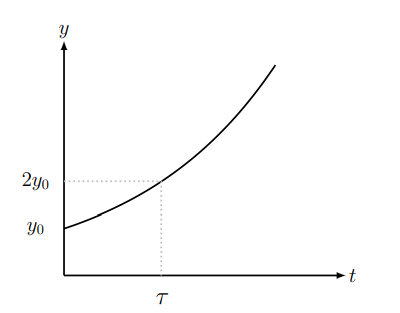
We summarize an important observation:

In general, an equation of the form

\[\frac{d y}{d t}=k y \nonumber \]

that represents an exponential growth has a doubling time of

\[\tau=\frac{\ln (2)}{k} . \nonumber \]

This is shown in Figure 11.6. We have discovered that based on the uncontrolled growth model, the population doubles every 55 years! After 110 years, for example, there have been two doublings, or a quadrupling of the population.

Figure 11.6: Doubling time for exponential growth.

Mastered Material Check

22. What are the units associated with \(\tau\) ?
23. The human population hit 3 billion in 1959. How does this fit with our (imperfect) model?

Example 11.6

(A ten year doubling time) Suppose we are told that some animal population doubles every 10 years. What growth rate would lead to such a trend?

Solution

In this case, \(\tau=10\) years. Rearranging

\[\tau=\frac{\ln (2)}{k}, \nonumber \]

we obtain

\[k=\frac{\ln (2)}{\tau}=\frac{0.6931}{10} \approx 0.07 \text { per year. } \nonumber \]

Thus, a growth rate of \(7 \%\) leads to doubling roughly every 10 years.