17.6: Appendix F- Trigonometry Review

The definition of trigonometric functions in terms of the angle \(\theta\) in a right triangle are reviewed in Figure. F.1.

Figure F.1: Review of the relation between ratios of side lengths (in a right triangle) and trigonometric functions of the associated angle.

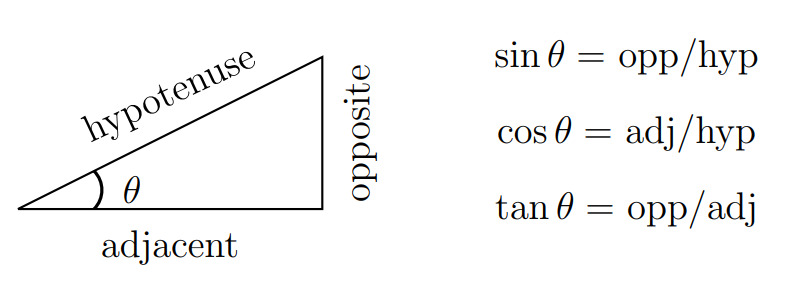
Based on these definitions, certain angles’ sine and cosine can be found explicitly - and similarly \(\tan (\theta)=\sin (\theta) / \cos (\theta)\). This is shown in Table F.1.

Table F.1: Values of the sines, cosines, and tangent for standard angles.

degrees	radians	\(\sin (\boldsymbol{t})\)	\(\cos (\boldsymbol{t})\)	\(\tan (\boldsymbol{t})\)
0	0	0	1	0
30	\(\frac{\pi}{6}\)	\(\frac{1}{2}\)	\(\frac{\sqrt{3}}{2}\)	\(\frac{1}{\sqrt{3}}\)
45	\(\frac{\pi}{4}\)	\(\frac{\sqrt{2}}{2}\)	\(\frac{\sqrt{2}}{2}\)	1
60	\(\frac{\pi}{3}\)	\(\frac{\sqrt{3}}{2}\)	\(\frac{1}{2}\)	\(\sqrt{3}\)
90	\(\frac{\pi}{2}\)	1	0	\(\infty\)

We also define the other trigonometric functions as follows:

\[\begin{aligned} & \tan (t)=\frac{\sin (t)}{\cos (t)}, \quad \cot (t)=\frac{1}{\tan (t)}, \\ & \sec (t)=\frac{1}{\cos (t)}, \quad \csc (t)=\frac{1}{\sin (t)} . \end{aligned} \nonumber \]

Sine and cosine are related by the identity

\[\cos (t)=\sin \left(t+\frac{\pi}{2}\right) . \nonumber \]

This identity then leads to two others of similar form. Dividing each side of the above relation by \(\cos ^{2}(t)\) yields

\[\tan ^{2}(t)+1=\sec ^{2}(t), \nonumber \]

whereas division by \(\sin ^{2}(t)\) gives us

\[1+\cot ^{2}(t)=\csc ^{2}(t) . \nonumber \]

These aid in simplifying expressions involving the trigonometric functions, as we shall see.

Law of cosines

This law relates the cosine of an angle to the lengths of sides formed in a triangle (see Figure F.2).

\[c^{2}=a^{2}+b^{2}-2 a b \cos (\theta) \nonumber \]

where the side of length \(c\) is opposite the angle \(\theta\).

Figure F.2: Law of cosines states that \(c^{2}=\) \(a^{2}+b^{2}-2 a b \cos (\theta)\).

There are other important relations between the trigonometric functions (called trigonometric identities). These should be remembered.

Angle sum identities

The trigonometric functions are nonlinear. This means that, for example, the sine of the sum of two angles is not just the sum of the two sines. One can use the law of cosines and other geometric ideas to establish the following two relationships:

\[\begin{aligned} & \sin (A+B)=\sin (A) \cos (B)+\sin (B) \cos (A) \\ & \cos (A+B)=\cos (A) \cos (B)-\sin (A) \sin (B) \end{aligned} \nonumber \]

These two identities appear in many calculations and aid in computing derivatives of basic trigonometric formulae.

Related identities. The identities for the sum of angles can be used to derive a number of related formulae. For example, by replacing \(B\) by \(-B\) we get the angle difference identities:

\[\begin{aligned} & \sin (A-B)=\sin (A) \cos (B)-\sin (B) \cos (A) \\ & \cos (A-B)=\cos (A) \cos (B)+\sin (A) \sin (B) \end{aligned} \nonumber \]

By setting \(\theta=A=B\), we find the subsidiary double angle formulae:

\[\begin{gathered} \sin (2 \theta)=2 \sin (\theta) \cos (\theta) \\ \cos (2 \theta)=\cos ^{2}(\theta)-\sin ^{2}(\theta) \end{gathered} \nonumber \]

and these can also be written in the form

\[\begin{aligned} & 2 \cos ^{2}(\theta)=1+\cos (2 \theta) \\ & 2 \sin ^{2}(\theta)=1-\cos (2 \theta) \end{aligned} \nonumber \]

F.1 Summary of the inverse trigonometric functions

In Table F. 2 we show the table of standard values of functions \(\arcsin (x)\) and \(\arccos (x)\). In Figure F.3 we summarize the the relationships between the original trigonometric functions and their inverses.

Table F.2: Standard values of the inverse trigonometric functions.

\(\boldsymbol{x}\)	\(\arcsin (\boldsymbol{x})\)	\(\arccos (\boldsymbol{x})\)
\(\hdashline-1\)	\(-\pi / 2\)	\(\pi\)
\(-\sqrt{3} / 2\)	\(-\pi / 3\)	\(5 \pi / 6\)
\(-\sqrt{2} / 2\)	\(-\pi / 4\)	\(3 \pi / 4\)
\(-1 / 2\)	\(-\pi / 6\)	\(2 \pi / 3\)
0	0	\(\pi / 2\)
\(1 / 2\)	\(\pi / 6\)	\(\pi / 3\)
\(\sqrt{2} / 2\)	\(\pi / 4\)	\(\pi / 4\)
\(\sqrt{3} / 2\)	\(\pi / 3\)	\(\pi / 6\)
1	\(\pi / 2\)	0

Figure F.3: A summary of the trigonometric functions and their inverses. (a) \(\operatorname{Sin}(x)\) (b) \(\arcsin (x)\), (b) \(\operatorname{Cos}(x)\) (d) \(\arccos (x)\), (e) \(\operatorname{Tan}(x)\) (f) \(\arctan (x)\). The red curves are the restricted domain portions of the original trig functions. The gold curves are the inverse functions.