2.E: Limits (Exercises)

Last updated
Save as PDF

Page ID: 17419

$ \newcommand{\vecs}[1]{\overset { \scriptstyle \rightharpoonup} {\mathbf{#1}} } $

$ \newcommand{\vecd}[1]{\overset{-\!-\!\rightharpoonup}{\vphantom{a}\smash {#1}}} $

$ \newcommand{\id}{\mathrm{id}}$ $ \newcommand{\Span}{\mathrm{span}}$

( \newcommand{\kernel}{\mathrm{null}\,}\) $ \newcommand{\range}{\mathrm{range}\,}$

$ \newcommand{\RealPart}{\mathrm{Re}}$ $ \newcommand{\ImaginaryPart}{\mathrm{Im}}$

$ \newcommand{\Argument}{\mathrm{Arg}}$ $ \newcommand{\norm}[1]{\| #1 \|}$

$ \newcommand{\inner}[2]{\langle #1, #2 \rangle}$

$ \newcommand{\Span}{\mathrm{span}}$

$ \newcommand{\id}{\mathrm{id}}$

$ \newcommand{\Span}{\mathrm{span}}$

$ \newcommand{\kernel}{\mathrm{null}\,}$

$ \newcommand{\range}{\mathrm{range}\,}$

$ \newcommand{\RealPart}{\mathrm{Re}}$

$ \newcommand{\ImaginaryPart}{\mathrm{Im}}$

$ \newcommand{\Argument}{\mathrm{Arg}}$

$ \newcommand{\norm}[1]{\| #1 \|}$

$ \newcommand{\inner}[2]{\langle #1, #2 \rangle}$

$ \newcommand{\Span}{\mathrm{span}}$ $ \newcommand{\AA}{\unicode[.8,0]{x212B}}$

$ \newcommand{\vectorA}[1]{\vec{#1}} % arrow$

$ \newcommand{\vectorAt}[1]{\vec{\text{#1}}} % arrow$

$ \newcommand{\vectorB}[1]{\overset { \scriptstyle \rightharpoonup} {\mathbf{#1}} } $

$ \newcommand{\vectorC}[1]{\textbf{#1}} $

$ \newcommand{\vectorD}[1]{\overrightarrow{#1}} $

$ \newcommand{\vectorDt}[1]{\overrightarrow{\text{#1}}} $

$ \newcommand{\vectE}[1]{\overset{-\!-\!\rightharpoonup}{\vphantom{a}\smash{\mathbf {#1}}}} $

$ \newcommand{\vecs}[1]{\overset { \scriptstyle \rightharpoonup} {\mathbf{#1}} } $

$ \newcommand{\vecd}[1]{\overset{-\!-\!\rightharpoonup}{\vphantom{a}\smash {#1}}} $

$\newcommand{\avec}{\mathbf a}$ $\newcommand{\bvec}{\mathbf b}$ $\newcommand{\cvec}{\mathbf c}$ $\newcommand{\dvec}{\mathbf d}$ $\newcommand{\dtil}{\widetilde{\mathbf d}}$ $\newcommand{\evec}{\mathbf e}$ $\newcommand{\fvec}{\mathbf f}$ $\newcommand{\nvec}{\mathbf n}$ $\newcommand{\pvec}{\mathbf p}$ $\newcommand{\qvec}{\mathbf q}$ $\newcommand{\svec}{\mathbf s}$ $\newcommand{\tvec}{\mathbf t}$ $\newcommand{\uvec}{\mathbf u}$ $\newcommand{\vvec}{\mathbf v}$ $\newcommand{\wvec}{\mathbf w}$ $\newcommand{\xvec}{\mathbf x}$ $\newcommand{\yvec}{\mathbf y}$ $\newcommand{\zvec}{\mathbf z}$ $\newcommand{\rvec}{\mathbf r}$ $\newcommand{\mvec}{\mathbf m}$ $\newcommand{\zerovec}{\mathbf 0}$ $\newcommand{\onevec}{\mathbf 1}$ $\newcommand{\real}{\mathbb R}$ $\newcommand{\twovec}[2]{\left[\begin{array}{r}#1 \\ #2 \end{array}\right]}$ $\newcommand{\ctwovec}[2]{\left[\begin{array}{c}#1 \\ #2 \end{array}\right]}$ $\newcommand{\threevec}[3]{\left[\begin{array}{r}#1 \\ #2 \\ #3 \end{array}\right]}$ $\newcommand{\cthreevec}[3]{\left[\begin{array}{c}#1 \\ #2 \\ #3 \end{array}\right]}$ $\newcommand{\fourvec}[4]{\left[\begin{array}{r}#1 \\ #2 \\ #3 \\ #4 \end{array}\right]}$ $\newcommand{\cfourvec}[4]{\left[\begin{array}{c}#1 \\ #2 \\ #3 \\ #4 \end{array}\right]}$ $\newcommand{\fivevec}[5]{\left[\begin{array}{r}#1 \\ #2 \\ #3 \\ #4 \\ #5 \\ \end{array}\right]}$ $\newcommand{\cfivevec}[5]{\left[\begin{array}{c}#1 \\ #2 \\ #3 \\ #4 \\ #5 \\ \end{array}\right]}$ $\newcommand{\mattwo}[4]{\left[\begin{array}{rr}#1 \amp #2 \\ #3 \amp #4 \\ \end{array}\right]}$ $\newcommand{\laspan}[1]{\text{Span}\{#1\}}$ $\newcommand{\bcal}{\cal B}$ $\newcommand{\ccal}{\cal C}$ $\newcommand{\scal}{\cal S}$ $\newcommand{\wcal}{\cal W}$ $\newcommand{\ecal}{\cal E}$ $\newcommand{\coords}[2]{\left\{#1\right\}_{#2}}$ $\newcommand{\gray}[1]{\color{gray}{#1}}$ $\newcommand{\lgray}[1]{\color{lightgray}{#1}}$ $\newcommand{\rank}{\operatorname{rank}}$ $\newcommand{\row}{\text{Row}}$ $\newcommand{\col}{\text{Col}}$ $\renewcommand{\row}{\text{Row}}$ $\newcommand{\nul}{\text{Nul}}$ $\newcommand{\var}{\text{Var}}$ $\newcommand{\corr}{\text{corr}}$ $\newcommand{\len}[1]{\left|#1\right|}$ $\newcommand{\bbar}{\overline{\bvec}}$ $\newcommand{\bhat}{\widehat{\bvec}}$ $\newcommand{\bperp}{\bvec^\perp}$ $\newcommand{\xhat}{\widehat{\xvec}}$ $\newcommand{\vhat}{\widehat{\vvec}}$ $\newcommand{\uhat}{\widehat{\uvec}}$ $\newcommand{\what}{\widehat{\wvec}}$ $\newcommand{\Sighat}{\widehat{\Sigma}}$ $\newcommand{\lt}{<}$ $\newcommand{\gt}{>}$ $\newcommand{\amp}{&}$ $\definecolor{fillinmathshade}{gray}{0.9}$

2.1: A Preview of Calculus

For exercises 1 - 3 , points $P(1,2)$ and $Q(x,y)$ are on the graph of the function $f(x)=x^2+1$.

1) [T] Complete the following table with the appropriate values: $y$-coordinate of $Q$, the point $Q(x,y)$, and the slope of the secant line passing through points $P$ and $Q$. Round your answer to eight significant digits.

$x$	$y$	$Q(x,y)$	$m_{sec}$
1.1	a.	e.	i.
1.01	b.	f.	j.
1.001	c.	g.	k.
1.0001	d.	h.	l.

Answer: a. 2.2100000
b. 2.0201000
c. 2.0020010
d. 2.0002000
e. (1.1000000, 2.2100000)
f. (1.0100000, 2.0201000)
g. (1.0010000, 2.0020010)
h. (1.0001000, 2.0002000)
i. 2.1000000
j. 2.0100000
k. 2.0010000
l. 2.0001000

2) Use the values in the right column of the table in the preceding exercise to guess the value of the slope of the line tangent to $f$ at $x=1$.

3) Use the value in the preceding exercise to find the equation of the tangent line at point $P$. Graph $f(x)$ and the tangent line.

Answer: $y=2x$

For the exercises 4-6, points $P(1,1)$ and $Q(x,y)$ are on the graph of the function $f(x)=x^3$.

4) [T] Complete the following table with the appropriate values: $y$-coordinate of $Q$, the point $Q(x,y)$, and the slope of the secant line passing through points $P$ and $Q$. Round your answer to eight significant digits.

$x$	$y$	$Q(x,y)$	$m_{sec}$
1.1	a.	e.	i.
1.01	b.	f.	j.
1.001	c.	g.	k.
1.0001	d.	h.	l.2

5) Use the values in the right column of the table in the preceding exercise to guess the value of the slope of the tangent line to $f$ at $x=1$.

Answer: $3$

6) Use the value in the preceding exercise to find the equation of the tangent line at point $P$. Graph $f(x)$ and the tangent line.

For the exercises 7 - 9, points $P(4,2)$ and $Q(x,y)$ are on the graph of the function $f(x)=\sqrt{x}$.

7) [T] Complete the following table with the appropriate values: $y$-coordinate of $Q$, the point $Q(x,y)$, and the slope of the secant line passing through points $P$ and $Q$. Round your answer to eight significant digits.

$x$	$y$	$Q(x,y)$	$m_{sec}$
4.1	a.	e.	i.
4.01	b.	f.	j.
4.001	c.	g.	k.
4.0001	d.	h.	l.

Answer: a. 2.0248457
b. 2.0024984
c. 2.0002500
d. 2.0000250
e. (4.1000000,2.0248457)
f. (4.0100000,2.0024984)
g. (4.0010000,2.0002500)
h. (4.00010000,2.0000250)
i. 0.24845673
j. 0.24984395
k. 0.24998438
l. 0.24999844

8) Use the values in the right column of the table in the preceding exercise to guess the value of the slope of the tangent line to $f$ at $x=4$.

9) Use the value in the preceding exercise to find the equation of the tangent line at point $P$.

Answer: $y=\frac{x}{4}+1$

For exercises 10 - 12, points $P(1.5,0)$ and $Q(ϕ,y)$ are on the graph of the function $f(ϕ)=\cos(πϕ)$.

10) [T] Complete the following table with the appropriate values: $y$-coordinate of $Q$, the point $Q(ϕ,y)$, and the slope of the secant line passing through points $P$ and $Q$. Round your answer to eight significant digits.

$x$	$y$	$Q(ϕ,y)$	$m_{sec}$
1.4	a.	e.	i.
1.49	b.	f.	j.
1.499	c.	g.	k.
1.4999	d.	h.	l.

11) Use the values in the right column of the table in the preceding exercise to guess the value of the slope of the tangent line to f at $ϕ=1.5$.

Answer: $ π $

12) Use the value in the preceding exercise to find the equation of the tangent line at point $P$.

For exercises 13 - 15, points $P(−1,−1)$ and $Q(x,y)$ are on the graph of the function $f(x)=\frac{1}{x}$.

13) [T] Complete the following table with the appropriate values: $y$-coordinate of $Q$, the point $Q(x,y)$, and the slope of the secant line passing through points $P$ and $Q$. Round your answer to eight significant digits.

$x$	$y$	$Q(x,y)$	$m_{sec}$
-1.05	a.	e.	i.
-1.01	b.	f.	j.
-1.005	c.	g.	k.
-1.001	d.	h.	l.

Answer: a. −0.95238095
b. −0.99009901
c. −0.99502488
d. −0.99900100
e. (−1;.0500000,−0;.95238095)
f. (−1;.0100000,−0;.9909901)
g. (−1;.0050000,−0;.99502488)
h. (1.0010000,−0;.99900100)
i. −0.95238095
j. −0.99009901
k. −0.99502488
l. −0.99900100

14) Use the values in the right column of the table in the preceding exercise to guess the value of the slope of the line tangent to $f$ at $x=−1$.

15) Use the value in the preceding exercise to find the equation of the tangent line at point $P$.

Answer: $y=−x−2$

For exercises 16 - 17, the position function of a ball dropped from the top of a 200-meter tall building is given by $s(t)=200−4.9t^2$, where position $s$ is measured in meters and time $t$ is measured in seconds. Round your answer to eight significant digits.

16) [T] Compute the average velocity of the ball over the given time intervals.

a. [4.99,5]

b. [5,5.01]

c. [4.999,5]

d. [5,5.001]

17) Use the preceding exercise to guess the instantaneous velocity of the ball at $t=5$ sec.

Answer: $−49$ m/sec (velocity of the ball is 49 m/sec downward)

For exercises 18 - 19, consider a stone tossed into the air from ground level with an initial velocity of 15 m/sec. Its height in meters at time $t$ seconds is $h(t)=15t−4.9t^2$.

18) [T] Compute the average velocity of the stone over the given time intervals.

a. [1,1.05]

b. [1,1.01]

c. [1,1.005]

d. [1,1.001]

19) Use the preceding exercise to guess the instantaneous velocity of the stone at $t=1$ sec.

Answer: $5.2$ m/sec

For exercises 20 - 21, consider a rocket shot into the air that then returns to Earth. The height of the rocket in meters is given by $h(t)=600+78.4t−4.9t^2$, where $t$ is measured in seconds.

20) [T] Compute the average velocity of the rocket over the given time intervals.

a. [9,9.01]

b. [8.99,9]

c. [9,9.001]

d. [8.999,9]

21) Use the preceding exercise to guess the instantaneous velocity of the rocket at $t=9$ sec.

Answer: $-9.8$ m/sec

For exercises, consider an athlete running a 40-m dash. The position of the athlete is given by $d(t)=\frac{t^3}{6}+4t$, where $d$ is the position in meters and $t$ is the time elapsed, measured in seconds.

22) [T] Compute the average velocity of the runner over the given time intervals.

a. [1.95,2.05]

b. [1.995,2.005]

c. [1.9995,2.0005]

d. [2,2.00001]

23) Use the preceding exercise to guess the instantaneous velocity of the runner at $t=2$ sec.

Answer: $6$ m/sec

For exercises 24 - 25, consider the function$f(x)=|x|$.

24) Sketch the graph of $f$ over the interval [$−1,2$] and shade the region above the $x$-axis.

25) Use the preceding exercise to find the exact value of the area between the $x$-axis and the graph of $f$ over the interval [$−1,2$] using rectangles. For the rectangles, use the square units, and approximate both above and below the lines. Use geometry to find the exact answer.

Answer: Under, 1 $unit^2$; over: 4 $unit^2$.
The exact area of the two triangles is $\frac{1}{2}(1)(1)+\frac{1}{2}(2)(2)=2.5 units^2$.

For exercises 26 - 27, consider the function $f(x)=\sqrt{1−x^2}$. (Hint: This is the upper half of a circle of radius 1 positioned at $(0,0)$.)

26) Sketch the graph of f over the interval [$−1,1$].

27) Use the preceding exercise to find the exact area between the $x$-axis and the graph of $f$ over the interval [$−1,1$] using rectangles. For the rectangles, use squares 0.4 by 0.4 units, and approximate both above and below the lines. Use geometry to find the exact answer.

Answer: Under, $0.96 \;\text{units}^2$; over, $1.92 \;\text{units}^2$).
The exact area of the semicircle with radius 1 is $\frac{π(1)^2}{2}=\frac{π}{2} \;\text{units}^2$

For exercises 28 - 29, consider the function $f(x)=−x^2+1$.

28) Sketch the graph of $f$ over the interval [$−1,1$].

29) Approximate the area of the region between the $x$-axis and the graph of $f$ over the interval [$−1,1$].

Answer: Approximately $1.3333333 \;\text{units}^2$

2.2: The Limit of a Function

Intuitive Definition of Limits

For exercises 1 - 2, consider the function $f(x)=\dfrac{x^2−1}{|x−1|}$.

1) [T] Complete the following table for the function. Round your solutions to four decimal places.

$x$	$f(x)$	$x$	$f(x)$
0.9	a.	1.1	e.
0.99	b.	1.01	f.
0.999	c.	1.001	g.
0.9999	d.	1.0001	h.

2) What do your results in the preceding exercise indicate about the two-sided limit $\displaystyle \lim_{x→1}f(x)$? Explain your response.

Answer: $\displaystyle \lim_{x \to 1}f(x)$ does not exist because $\displaystyle \lim_{x \to 1^−}f(x)=−2≠\lim_{x \to 1^+}f(x)=2$.

For exercises 3 - 5, consider the function $f(x)=(1+x)^{1/x}$.

3) [T] Make a table showing the values of $f$ for $x=−0.01,\;−0.001,\;−0.0001,\;−0.00001$ and for $x=0.01,\;0.001,\;0.0001,\;0.00001$. Round your solutions to five decimal places.

$x$	$f(x)$	$x$	$f(x)$
-0.01	a.	0.01	e.
-0.001	b.	0.001	f.
-0.0001	c.	0.0001	g.
-0.00001	d.	0.00001	h.

4) What does the table of values in the preceding exercise indicate about the function $f(x)=(1+x)^{1/x}$?

Answer: $\displaystyle \lim_{x \to 0}(1+x)^{1/x}\approx 2.7183$.

5) To which mathematical constant do the values in the preceding exercise appear to be approaching? This is the actual limit here.

In exercises 6 - 8, use the given values to set up a table to evaluate the limits. Round your solutions to eight decimal places.

6) [T] $\displaystyle \lim_{x \to 0}\frac{\sin 2x}{x};\quad ±0.1,\; ±0.01, \; ±0.001, \;±.0001$

$x$	$\frac{\sin 2x}{x}$	$x$	$\frac{\sin 2x}{x}$
-0.1	a.	0.1	e.
-0.01	b.	0.01	f.
-0.001	c.	0.001	g.
-0.0001	d.	0.0001	h.

Answer: a. 1.98669331; b. 1.99986667; c. 1.99999867; d. 1.99999999; e. 1.98669331; f. 1.99986667; g. 1.99999867; h. 1.99999999;
$\displaystyle \lim_{x \to 0}\frac{\sin 2x}{x}=2$

7) [T] $\displaystyle \lim_{x \to 0}\frac{\sin 3x}{x} ±0.1, \; ±0.01, \; ±0.001, \; ±0.0001$

$x$	$\frac{\sin 3x}{x}$	$x$	$\frac{\sin 3x}{x}$
-0.1	a.	0.1	e.
-0.01	b.	0.01	f.
-0.001	c.	0.001	g.
-0.0001	d.	0.0001	h.

8) Use the preceding two exercises to conjecture (guess) the value of the following limit: $\displaystyle \lim_{x \to 0}\frac{\sin ax}{x}$ for $a$, a positive real value.

Answer: $\displaystyle \lim_{x \to 0}\frac{\sin ax}{x}=a$

[T] In exercises 9 - 14, set up a table of values to find the indicated limit. Round to eight significant digits.

9) $\displaystyle \lim_{x \to 2}\frac{x^2−4}{x^2+x−6}$

$x$	$\frac{x^2−4}{x^2+x−6}$	$x$	$\frac{x^2−4}{x^2+x−6}$
1.9	a.	2.1	e.
1.99	b.	2.01	f.
1.999	c.	2.001	g.
1.9999	d.	2.0001	h.

10) $\displaystyle \lim_{x \to 1}(1−2x)$

$x$	$1−2x$	$x$	$1−2x$
0.9	a.	1.1	e.
0.99	b.	1.01	f.
0.999	c.	1.001	g.
0.9999	d.	1.0001	h.

Answer: a. −0.80000000; b. −0.98000000; c. −0.99800000; d. −0.99980000; e. −1.2000000; f. −1.0200000; g. −1.0020000; h. −1.0002000;
$ \displaystyle \lim_{x \to 1}(1−2x)=−1$

11) $\displaystyle \lim_{x \to 0}\frac{5}{1−e^{1/x}}$

$x$	$\frac{5}{1−e^{1/x}}$	$x$	$\frac{5}{1−e^{1/x}}$
-0.1	a.	0.1	e.
-0.01	b.	0.01	f.
-0.001	c.	0.001	g.
-0.0001	d.	0.0001	h.

12) $\displaystyle \lim_{z \to 0}\frac{z−1}{z^2(z+3)}$

$z$	$\frac{z−1}{z^2(z+3)}$	$z$	$\frac{z−1}{z^2(z+3)}$
-0.1	a.	0.1	e.
-0.01	b.	0.01	f.
-0.001	c.	0.001	g.
-0.0001	d.	0.0001	h.

Answer: a. −37.931034; b. −3377.9264; c. −333,777.93; d. −33,337,778; e. −29.032258; f. −3289.0365; g. −332,889.04; h. −33,328,889
$ \displaystyle \lim_{x \to 0}\frac{z−1}{z^2(z+3)}=−∞$

13) $\displaystyle \lim_{t \to 0^+}\frac{\cos t}{t}$

$t$	$\frac{\cos t}{t}$
0.1	a.
0.01	b.
0.001	c.
0.0001	d.

14) $\displaystyle \lim_{x \to 2}\frac{1−\frac{2}{x}}{x^2−4}$

$x$	$\frac{1−\frac{2}{x}}{x^2−4}$	$x$	$\frac{1−\frac{2}{x}}{x^2−4}$
1.9	a.	2.1	e.
1.99	b.	2.01	f.
1.999	c.	2.001	g.
1.9999	d.	2.0001	h.

Answer: a. 0.13495277; b. 0.12594300; c. 0.12509381; d. 0.12500938; e. 0.11614402; f. 0.12406794; g. 0.12490631; h. 0.12499063;
$ \displaystyle ∴\lim_{x \to 2}\frac{1−\frac{2}{x}}{x^2−4}=0.1250=\frac{1}{8}$

[T] In exercises 15 - 16, set up a table of values and round to eight significant digits. Based on the table of values, make a guess about what the limit is. Then, use a calculator to graph the function and determine the limit. Was the conjecture correct? If not, why does the method of tables fail?

15) $\displaystyle \lim_{θ \to 0}\sin\left(\frac{π}{θ}\right)$

$θ$	$\sin\left(\frac{π}{θ}\right)$	$θ$	$\sin\left(\frac{π}{θ}\right)$
-0.1	a.	0.1	e.
-0.01	b.	0.01	f.
-0.001	c.	0.001	g.
-0.0001	d.	0.0001	h.

16) $\displaystyle \lim_{α \to 0^+} \frac{1}{α}\cos\left(\frac{π}{α}\right)$

$a$	$\frac{1}{α}\cos\left(\frac{π}{α}\right)$
0.1	a.
0.01	b.
0.001	c.
0.0001	d.

Answer

a. 10.00000; b. 100.00000; c. 1000.0000; d. 10,000.000;
Guess: $\displaystyle \lim_{α→0^+}\frac{1}{α}\cos\left(\frac{π}{α}\right)=∞$;
Actual: DNE , since the graph shows the function oscillates wildly between values approaching positive infinity and values approaching negative infinity, as the value of $α$ approaches $0$ from the positive side.

$A graph of the function (1/alpha) * cos (pi / alpha), which oscillates gently until the interval [-.2, .2], where it oscillates rapidly, going to infinity and negative infinity as it approaches the y axis.$

In exercises 17 - 20, consider the graph of the function $y=f(x)$ shown here. Which of the statements about $y=f(x)$ are true and which are false? Explain why a statement is false.

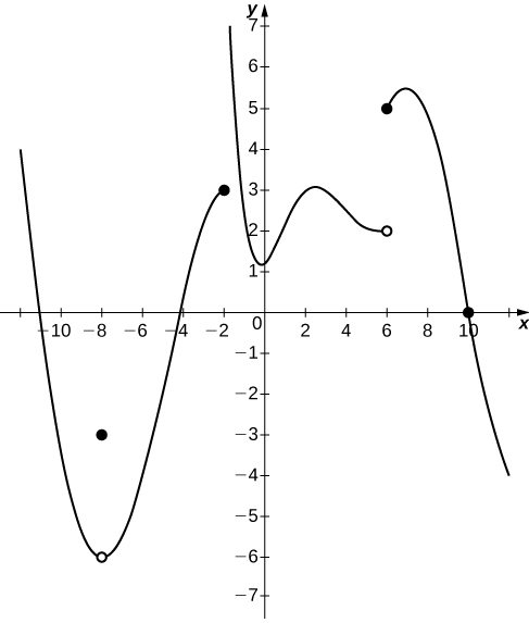
$A graph of a piecewise function with three segments and a point. The first segment is a curve opening upward with vertex at (-8, -6). This vertex is an open circle, and there is a closed circle instead at (-8, -3). The segment ends at (-2,3), where there is a closed circle. The second segment stretches up asymptotically to infinity along x=-2, changes direction to increasing at about (0,1.25), increases until about (2.25, 3), and decreases until (6,2), where there is an open circle. The last segment starts at (6,5), increases slightly, and then decreases into quadrant four, crossing the x axis at (10,0). All of the changes in direction are smooth curves.$

17) $\displaystyle \lim_{x→10}f(x)=0$

18) $\displaystyle \lim_{x→−2^+}f(x)=3$

Answer: False; $\displaystyle \lim_{x→−2^+}f(x)=+∞$

19) $\displaystyle \lim_{x→−8}f(x)=f(−8)$

20) $\displaystyle \lim_{x→6}f(x)=5$

Answer: False; $\displaystyle \lim_{x→6}f(x)$ DNE since $\displaystyle \lim_{x→6^−}f(x)=2$ and $\displaystyle \lim_{x→6^+}f(x)=5$.

In exercises 21 - 25, use the following graph of the function $y=f(x)$ to find the values, if possible. Estimate when necessary.

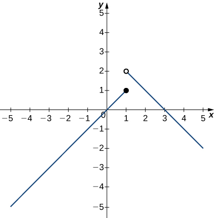
$A graph of a piecewise function with two segments. The first segment exists for x <=1, and the second segment exists for x > 1. The first segment is linear with a slope of 1 and goes through the origin. Its endpoint is a closed circle at (1,1). The second segment is also linear with a slope of -1. It begins with the open circle at (1,2).$

21) $\displaystyle \lim_{x→1^−}f(x)$

22) $\displaystyle \lim_{x→1^+}f(x)$

Answer: $2$

23) $\displaystyle \lim_{x→1}f(x)$

24) $\displaystyle \lim_{x→2}f(x)$

Answer: $1$

25) $f(1)$

In exercises 26 - 29, use the graph of the function $y=f(x)$ shown here to find the values, if possible. Estimate when necessary.

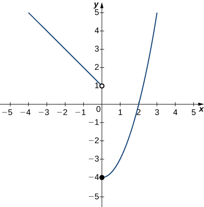
$A graph of a piecewise function with two segments. The first is a linear function for x < 0. There is an open circle at (0,1), and its slope is -1. The second segment is the right half of a parabola opening upward. Its vertex is a closed circle at (0, -4), and it goes through the point (2,0).$

26) $\displaystyle \lim_{x→0^−}f(x)$

Answer: $1$

27) $\displaystyle \lim_{x→0^+}f(x)$

28) $\displaystyle \lim_{x→0}f(x)$

Answer: DNE

29) $\displaystyle \lim_{x→2}f(x)$

In exercises 30 - 35, use the graph of the function $y=f(x)$ shown here to find the values, if possible. Estimate when necessary.

$A graph of a piecewise function with three segments, all linear. The first exists for x < -2, has a slope of 1, and ends at the open circle at (-2, 0). The second exists over the interval [-2, 2], has a slope of -1, goes through the origin, and has closed circles at its endpoints (-2, 2) and (2,-2). The third exists for x>2, has a slope of 1, and begins at the open circle (2,2).$

30) $\displaystyle \lim_{x→−2^−}f(x)$

Answer: $0$

31) $\displaystyle \lim_{x→−2^+}f(x)$

32) $\displaystyle \lim_{x→−2}f(x)$

Answer: DNE

33) $\displaystyle \lim_{x→2^−}f(x)$

34) $\displaystyle \lim_{x→2^+}f(x)$

Answer: $2$

35) $\displaystyle \lim_{x→2}f(x)$

In exercises 36 - 38, use the graph of the function $y=g(x)$ shown here to find the values, if possible. Estimate when necessary.

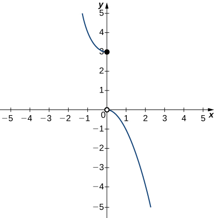
$A graph of a piecewise function with two segments. The first exists for x>=0 and is the left half of an upward opening parabola with vertex at the closed circle (0,3). The second exists for x>0 and is the right half of a downward opening parabola with vertex at the open circle (0,0).$

36) $\displaystyle \lim_{x→0^−}g(x)$

Answer: $3$

37) $\displaystyle \lim_{x→0^+}g(x)$

38) $\displaystyle \lim_{x→0}g(x)$

Answer: DNE

In exercises 39 - 41, use the graph of the function $y=h(x)$ shown here to find the values, if possible. Estimate when necessary.

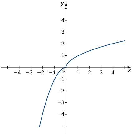
$A graph of a function with two curves approaching 0 from quadrant 1 and quadrant 3. The curve in quadrant one appears to be the top half of a parabola opening to the right of the y axis along the x axis with vertex at the origin. The curve in quadrant three appears to be the left half of a parabola opening downward with vertex at the origin.$

39) $\displaystyle \lim_{x→0^−}h(x)$

40) $\displaystyle \lim_{x→0^+}h(x)$

Answer: $0$

41) $\displaystyle \lim_{x→0}h(x)$

In exercises 42 - 46, use the graph of the function $y=f(x)$ shown here to find the values, if possible. Estimate when necessary.

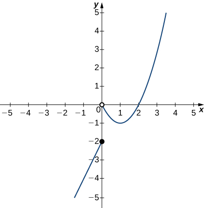
$A graph with a curve and a point. The point is a closed circle at (0,-2). The curve is part of an upward opening parabola with vertex at (1,-1). It exists for x > 0, and there is a closed circle at the origin.$

42) $\displaystyle \lim_{x→0^−}f(x)$

Answer: $-2$

43) $\displaystyle \lim_{x→0^+}f(x)$

44) $\displaystyle \lim_{x→0}f(x)$

Answer: DNE

45) $\displaystyle \lim_{x→1}f(x)$

46) $\displaystyle \lim_{x→2}f(x)$

Answer: $0$

Infinite Limits

In exercises 47 - 51, sketch the graph of a function with the given properties.

47) $\displaystyle \lim_{x→2}f(x)=1, \quad \lim_{x→4^−}f(x)=3, \quad \lim_{x→4^+}f(x)=6, \quad x=4$ is not defined.

48) $\displaystyle \lim_{x→−∞}f(x)=0, \quad \lim_{x→−1^−}f(x)=−∞, \quad \lim_{x→−1^+}f(x)=∞,\quad \lim_{x→0}f(x)=f(0), \quad f(0)=1, \quad \lim_{x→∞}f(x)=−∞$

Answer

Answers may vary

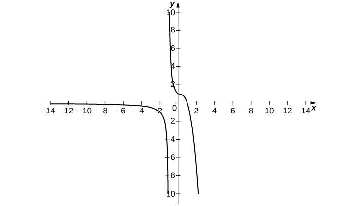
$A graph of a piecewise function with two segments. The first segment is in quadrant three and asymptotically goes to negative infinity along the y axis and 0 along the x axis. The second segment consists of two curves. The first appears to be the left half of an upward opening parabola with vertex at (0,1). The second appears to be the right half of a downward opening parabola with vertex at (0,1) as well.$

49) $\displaystyle \lim_{x→−∞}f(x)=2, \quad \lim_{x→3^−}f(x)=−∞, \quad \lim_{x→3^+}f(x)=∞, \quad \lim_{x→∞}f(x)=2, \quad f(0)=-\frac{1}{3}$

50) $\displaystyle \lim_{x→−∞}f(x)=2,\quad \lim_{x→−2}f(x)=−∞,\quad \lim_{x→∞}f(x)=2,\quad f(0)=0$

Answer

Answer may vary

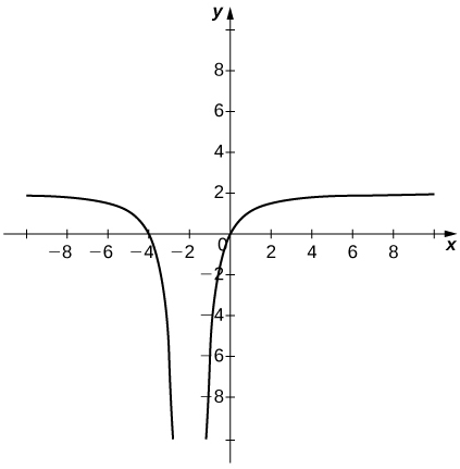
$A graph containing two curves. The first goes to 2 asymptotically along y=2 and to negative infinity along x = -2. The second goes to negative infinity along x=-2 and to 2 along y=2.$

51) $\displaystyle \lim_{x→−∞}f(x)=0,\quad \lim_{x→−1^−}f(x)=∞,\quad \lim_{x→−1^+}f(x)=−∞, \quad f(0)=−1, \quad \lim_{x→1^−}f(x)=−∞, \quad \lim_{x→1^+}f(x)=∞, \quad \lim_{x→∞}f(x)=0$

52) Shock waves arise in many physical applications, ranging from supernovas to detonation waves. A graph of the density of a shock wave with respect to distance, $x$, is shown here. We are mainly interested in the location of the front of the shock, labeled $X_{SF}$ in the diagram.

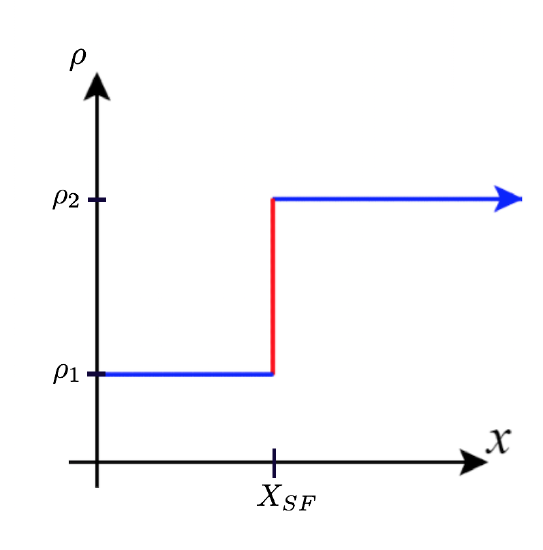
$A graph in quadrant one of the density of a shockwave with three labeled points: p1 and p2 on the y axis, with p1 > p2, and xsf on the x axis. It consists of y= p1 from 0 to xsf, x = xsf from y= p1 to y=p2, and y=p2 for values greater than or equal to xsf.$

a. Evaluate $\displaystyle \lim_{x→X_{SF}^+}ρ(x)$.

b. Evaluate $\displaystyle \lim_{x→X_{SF}^−}ρ(x)$.

c. Evaluate $\displaystyle \lim_{x→X_{SF}}ρ(x)$. Explain the physical meanings behind your answers.

Answer: a. $ρ_2$ b. $ρ_1$ c. DNE unless $ρ_1=ρ_2$. As you approach $X_{SF}$ from the right, you are in the high-density area of the shock. When you approach from the left, you have not experienced the “shock” yet and are at a lower density.

53) A track coach uses a camera with a fast shutter to estimate the position of a runner with respect to time. A table of the values of position of the athlete versus time is given here, where $x$ is the position in meters of the runner and $t$ is time in seconds. What is $\displaystyle \lim_{t→2}x(t)$? What does it mean physically?

$t(sec)$	$x(m)$
1.75	4.5
1.95	6.1
1.99	6.42
2.01	6.58
2.05	6.9
2.25	8.5

2.3: The Limit Laws

In exercises 1 - 4, use the limit laws to evaluate each limit. Justify each step by indicating the appropriate limit law(s).

1) $\displaystyle \lim_{x→0}\,(4x^2−2x+3)$

Answer

Use constant multiple law and difference law:

$\displaystyle \lim_{x→0}\,(4x^2−2x+3)=4\lim_{x→0}x^2−2\lim_{x→0}x+\lim_{x→0}3=0 + 0 + 3=3$

2) $\displaystyle \lim_{x→1}\frac{x^3+3x^2+5}{4−7x}$

3) $\displaystyle \lim_{x→−2}\sqrt{x^2−6x+3}$

Answer: Use root law: $\displaystyle \lim_{x→−2}\sqrt{x^2−6x+3}=\sqrt{\lim_{x→−2}(x^2−6x+3)}=\sqrt{19}$

4) $\displaystyle \lim_{x→−1}(9x+1)^2$

In exercises 5 - 10, use direct substitution to evaluate the limit of each continuous function.

5) $\displaystyle \lim_{x→7}x^2$

Answer: $\displaystyle \lim_{x→7}x^2\;=\;49$

6) $\displaystyle \lim_{x→−2}(4x^2−1)$

7) $\displaystyle \lim_{x→0}\frac{1}{1+\sin x}$

Answer: $\displaystyle \lim_{x→0}\frac{1}{1+\sin x}\;=\;1$

8) $\displaystyle \lim_{x→2}e^{2x−x^2}$

9) $\displaystyle \lim_{x→1}\frac{2−7x}{x+6}$

Answer: $\displaystyle \lim_{x→1}\frac{2−7x}{x+6}\;=\;−\frac{5}{7}$

10) $\displaystyle \lim_{x→3}\ln e^{3x}$

In exercises 11 - 20, use direct substitution to show that each limit leads to the indeterminate form $0/0$. Then, evaluate the limit analytically.

11) $\displaystyle \lim_{x→4}\frac{x^2−16}{x−4}$

Answer: $\displaystyle \text{When }x = 4, \quad\frac{x^2−16}{x−4}=\frac{16−16}{4−4}=\frac{0}{0};$

then, $\displaystyle \lim_{x→4}\frac{x^2−16}{x−4}= \lim_{x→4}\frac{(x+4)(x−4)}{x−4}=\lim_{x→4}(x+4) = 4+4 =8$

12) $\displaystyle \lim_{x→2}\frac{x−2}{x^2−2x}$

13) $\displaystyle \lim_{x→6}\frac{3x−18}{2x−12}$

Answer: $\displaystyle \text{When }x = 6, \quad\frac{3x−18}{2x−12}=\frac{18−18}{12−12}=\frac{0}{0};$

then, $\displaystyle \lim_{x→6}\frac{3x−18}{2x− 12}=\lim_{x→6}\frac{3(x−6)}{2(x−6)}=\lim_{x→6}\frac{3}{2}=\frac{3}{2}$

14) $\displaystyle \lim_{h→0}\frac{(1+h)^2−1}{h}$

15) $\displaystyle \lim_{t→9}\frac{t−9}{\sqrt{t}−3}$

Answer: $\displaystyle \text{When }t = 9, \quad\frac{t−9}{\sqrt{t}−3}=\frac{9−9}{3−3}=\frac{0}{0};$

then, $\displaystyle \lim_{t→9}\frac{t−9}{\sqrt{t}−3} =\lim_{t→9}\frac{t−9}{\sqrt{t}−3}\frac{\sqrt{t}+3}{\sqrt{t}+3}=\lim_{t→9}\frac{(t−9)(\sqrt{t}+3)}{t - 9}=\lim_{t→9}(\sqrt{t}+3)=\sqrt{9}+3=6$

16) $\displaystyle \lim_{h→0}\frac{\dfrac{1}{a+h}−\dfrac{1}{a}}{h}$, where $a$ is a real-valued constant

17) $\displaystyle \lim_{θ→π}\frac{\sin θ}{\tan θ}$

Answer: $\displaystyle \text{When }θ = π, \quad\frac{\sin θ}{\tan θ}=\frac{\sin π}{\tan π}=\frac{0}{0};$

then, $\displaystyle \lim_{θ→π}\frac{\sin θ}{\tan θ}=\lim_{θ→ π}\frac{\sin θ}{\frac{\sin θ}{\cos θ}}=\lim_{θ→π}\cos θ=\cos π=−1$

18) $\displaystyle \lim_{x→1}\frac{x^3−1}{x^2−1}$

19) $\displaystyle \lim_{x→1/2}\frac{2x^2+3x−2}{2x−1}$

Answer: $\displaystyle \text{When }x=1/2, \quad\frac{2x^2+3x−2}{2x−1}=\frac{\frac{1}{2}+\frac{3}{2}−2}{1−1}=\frac{0}{0};$

then, $\displaystyle \lim_{x→ 1/2}\frac{2x^2+3x−2}{2x−1}=\lim_{x→1/2}\frac{(2x−1)(x+2)}{2x−1}=\lim_{x→1/2}(x+2)=\frac{1}{2}+2=\frac{5}{2}$

20) $\displaystyle \lim_{x→−3}\frac{\sqrt{x+4}−1}{x+3}$

In exercises 21 - 24, use direct substitution to obtain an undefined expression. Then, use the method used in Example 9 of this section to simplify the function and determine the limit.

21) $\displaystyle \lim_{x→−2^−}\frac{2x^2+7x−4}{x^2+x−2}$

Answer: $−∞$

22) $\displaystyle \lim_{x→−2^+}\frac{2x^2+7x−4}{x^2+x−2}$

23) $\displaystyle \lim_{x→1^−}\frac{2x^2+7x−4}{x^2+x−2}$

Answer: $−∞$

24) $\displaystyle \lim_{x→1^+}\frac{2x^2+7x−4}{x^2+x−2}$

In exercises 25 - 32, assume that $\displaystyle \lim_{x→6}f(x)=4,\quad \lim_{x→6}g(x)=9$, and $\displaystyle \lim_{x→6}h(x)=6$. Use these three facts and the limit laws to evaluate each limit.

25) $\displaystyle \lim_{x→6}2f(x)g(x)$

Answer: $\displaystyle \lim_{x→6}2f(x)g(x)=2\left(\lim_{x→6}f(x)\right)\left(\lim_{x→6}g(x)\right)=2 (4)(9)=72$

26) $\displaystyle \lim_{x→6}\frac{g(x)−1}{f(x)}$

27) $\displaystyle \lim_{x→6}\left(f(x)+\frac{1}{3}g(x)\right)$

Answer: $\displaystyle \lim_{x→6}\left(f(x)+\frac{1}{3}g(x)\right)=\lim_{x→6}f(x)+\frac{1}{3}\lim_{x→6}g(x)=4+\frac{1}{3}(9)=7$

28) $\displaystyle \lim_{x→6}\frac{\big(h(x)\big)^3}{2}$

29) $\displaystyle \lim_{x→6}\sqrt{g(x)−f(x)}$

Answer: $\displaystyle \lim_{x→6}\sqrt{g(x)−f(x)}=\sqrt{\lim_{x→6}g(x)−\lim_{x→6}f(x)}=\sqrt{9-4}=\sqrt{5}$

30) $\displaystyle \lim_{x→6}x⋅h(x)$

31) $\displaystyle \lim_{x→6}[(x+1)⋅f(x)]$

Answer: $\displaystyle \lim_{x→6}[(x+1)f(x)]=\left(\lim_{x→6}(x+1)\right)\left(\lim_{x→6}f(x)\right)=7(4)=28$

32) $\displaystyle \lim_{x→6}(f(x)⋅g(x)−h(x))$

[T] In exercises 33 - 35, use a calculator to draw the graph of each piecewise-defined function and study the graph to evaluate the given limits.

33) $f(x)=\begin{cases}x^2, & x≤3\\ x+4, & x>3\end{cases}$

a. $\displaystyle \lim_{x→3^−}f(x)$

b. $\displaystyle \lim_{x→3^+}f(x)$

Answer

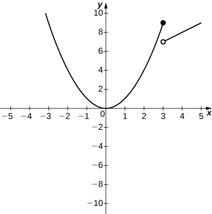
$The graph of a piecewise function with two segments. The first is the parabola x^2, which exists for x<=3. The vertex is at the origin, it opens upward, and there is a closed circle at the endpoint (3,9). The second segment is the line x+4, which is a linear function existing for x > 3. There is an open circle at (3, 7), and the slope is 1.$

a. $9$; b.$ 7$

34) $g(x)=\begin{cases}x^3−1, & x≤0\\1, & x>0\end{cases}$

a. $\displaystyle \lim_{x→0^−}g(x)$

b. $\displaystyle \lim_{x→0^+}g(x)$

35) $h(x)=\begin{cases}x^2−2x+1, & x<2\\3−x, & x≥2\end{cases}$

a. $\displaystyle \lim_{x→2^−}h(x)$

b. $\displaystyle \lim_{x→2^+}h(x)$

In exercises 36 - 43, use the following graphs and the limit laws to evaluate each limit.

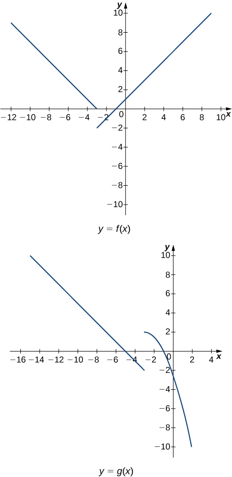
$Two graphs of piecewise functions. The upper is f(x), which has two linear segments. The first is a line with negative slope existing for x < -3. It goes toward the point (-3,0) at x= -3. The next has increasing slope and goes to the point (-3,-2) at x=-3. It exists for x > -3. Other key points are (0, 1), (-5,2), (1,2), (-7, 4), and (-9,6). The lower piecewise function has a linear segment and a curved segment. The linear segment exists for x < -3 and has decreasing slope. It goes to (-3,-2) at x=-3. The curved segment appears to be the right half of a downward opening parabola. It goes to the vertex point (-3,2) at x=-3. It crosses the y axis a little below y=-2. Other key points are (0, -7/3), (-5,0), (1,-5), (-7, 2), and (-9, 4).$

36) $\displaystyle \lim_{x→−3^+}(f(x)+g(x))$

37) $\displaystyle \lim_{x→−3^−}(f(x)−3g(x))$

Answer: $\displaystyle \lim_{x→−3^−}(f(x)−3g(x))=\lim_{x→−3^−}f(x)−3\lim_{x→−3^−}g(x)=0+6=6$

38) $\displaystyle \lim_{x→0}\frac{f(x)g(x)}{3}$

39) $\displaystyle \lim_{x→−5}\frac{2+g(x)}{f(x)}$

Answer: $\displaystyle \lim_{x→−5}\frac{2+g(x)}{f(x)}=\frac{2+\left(\displaystyle \lim_{x→−5}g(x)\right)}{\displaystyle \lim_{x→−5}f(x)}=\frac{2+0}{2}=1$

40) $\displaystyle \lim_{x→1}(f(x))^2$

41) $\displaystyle \lim_{x→1}\sqrt[3]{f(x)−g(x)}$

Answer: $\displaystyle \lim_{x→1}\sqrt[3]{f(x)−g(x)}=\sqrt[3]{\lim_{x→1}f(x)−\lim_{x→1}g(x)}=\sqrt[3]{2+5}=\sqrt[3]{7}$

42) $\displaystyle \lim_{x→−7}(x⋅g(x))$

43) $\displaystyle \lim_{x→−9}[x⋅f(x)+2⋅g(x)]$

Answer: $\displaystyle \lim_{x→−9}(xf(x)+2g(x))=\left(\lim_{x→−9}x\right)\left(\lim_{x→−9}f(x)\right)+2\lim_{x→−9}g(x)=(−9)(6)+2(4)=−46$

For exercises 44 - 46, evaluate the limit using the squeeze theorem. Use a calculator to graph the functions $f(x)$, $g(x)$, and $h(x)$ when possible.

44) [T] True or False? If $2x−1≤g(x)≤x^2−2x+3$, then $\displaystyle \lim_{x→2}g(x)=0$.

45) [T] $\displaystyle \lim_{θ→0}θ^2\cos\left(\frac{1}{θ}\right)$

Answer

The limit is zero.

$The graph of three functions over the domain [-1,1], colored red, green, and blue as follows: red: theta^2, green: theta^2 * cos (1/theta), and blue: - (theta^2). The red and blue functions open upwards and downwards respectively as parabolas with vertices at the origin. The green function is trapped between the two.$

46) $\displaystyle \lim_{x→0}f(x)$, where $f(x)=\begin{cases}0, & x\text{ rational}\\ x^2, & x\text{ irrrational}\end{cases}$

47) [T] In physics, the magnitude of an electric field generated by a point charge at a distance $r$ in vacuum is governed by Coulomb’s law: $E(r)=\dfrac{q}{4πε_0r^2}$, where $E$ represents the magnitude of the electric field, $q$ is the charge of the particle, $r$ is the distance between the particle and where the strength of the field is measured, and $\dfrac{1}{4πε_0}$ is Coulomb’s constant: $8.988×109N⋅m^2/C^2$.

a. Use a graphing calculator to graph $E(r)$ given that the charge of the particle is $q=10^{−10}$.

b. Evaluate $\displaystyle \lim_{r→0^+}E(r)$. What is the physical meaning of this quantity? Is it physically relevant? Why are you evaluating from the right?

Answer

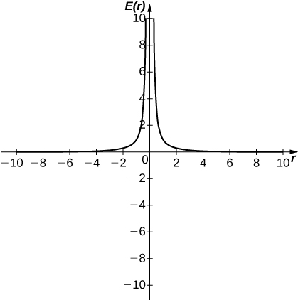
$A graph of a function with two curves. The first is in quadrant two and curves asymptotically to infinity along the y axis and to 0 along the x axis as x goes to negative infinity. The second is in quadrant one and curves asymptotically to infinity along the y axis and to 0 along the x axis as x goes to infinity.$

b. ∞. The magnitude of the electric field as you approach the particle q becomes infinite. It does not make physical sense to evaluate negative distance.

48) [T] The density of an object is given by its mass divided by its volume: $ρ=m/V.$

a. Use a calculator to plot the volume as a function of density $(V=m/ρ)$, assuming you are examining something of mass $8$ kg ($m=8$).

b. Evaluate $\displaystyle \lim_{x→0^+}V(\rho)$ and explain the physical meaning.

2.4: Continuity

For exercises 1 - 8, determine the point(s), if any, at which each function is discontinuous. Classify any discontinuity as jump, removable, infinite, or other.

1) $f(x)=\dfrac{1}{\sqrt{x}}$

Answer: The function is defined for all $x$ in the interval $(0,∞)$.

2) $f(x)=\dfrac{2}{x^2+1}$

3) $f(x)=\dfrac{x}{x^2−x}$

Answer: Removable discontinuity at $x=0$; infinite discontinuity at $x=1$.

4) $g(t)=t^{−1}+1$

5) $f(x)=\dfrac{5}{e^x−2}$

Answer: Infinite discontinuity at $x=\ln 2$

6) $f(x)=\dfrac{|x−2|}{x−2}$

7) $H(x)=\tan 2x$

Answer: Infinite discontinuities at $x=\dfrac{(2k+1)π}{4}$, for $k=0,\,±1,\,±2,\,±3,\,…$

8) $f(t)=\dfrac{t+3}{t^2+5t+6}$

For exercises 9 - 14, decide if the function continuous at the given point. If it is discontinuous, what type of discontinuity is it?

9) $\dfrac{2x^2−5x+3}{x−1}$ at $x=1$

Answer: No. It is a removable discontinuity.

10) $h(θ)=\dfrac{\sin θ−\cos θ}{\tan θ}$ at $θ=π$

11) $g(u)=\begin{cases}\dfrac{6u^2+u−2}{2u−1}, & \text{if }u≠ \frac{1}{2} \\ \frac{7}{2}, & \text{if }u= \frac{1}{2} \end{cases}$, at $u=\frac{1}{2}$

Answer: Yes. It is continuous.

12) $f(y)=\dfrac{\sin(πy)}{\tan(πy)}$, at $y=1$

13) $f(x)=\begin{cases}x^2−e^x, & \text{if } x<0\\x−1, & \text{if }x≥0\end{cases}$, at $x=0$

Answer: Yes. It is continuous.

14) $f(x)=\begin{cases}x\sin(x), & \text{if }x≤π\\ x\tan(x), & \text{if }x>π\end{cases}$, at $x=π$

In exercises 15 - 19, find the value(s) of $k$ that makes each function continuous over the given interval.

15) $f(x)=\begin{cases}3x+2, & \text{if }x<k\\2x−3, & \text{if }k≤x≤8\end{cases}$

Answer: $k=−5$

16) $f(θ)=\begin{cases}\sin θ, & \text{if }0≤θ<\frac{π}{2}\\ \cos(θ+k), & \text{if }\frac{π}{2}≤θ≤π\end{cases}$

17) $f(x)=\begin{cases}\dfrac{x^2+3x+2}{x+2}, & \text{if }x≠−2\\ k, & \text{if }x=−2\end{cases}$

Answer: $k=−1$

18) $f(x)=\begin{cases}e^{kx}, & \text{if }0≤x<4\\x+3, & \text{if }4≤x≤8\end{cases}$

19) $f(x)=\begin{cases}\sqrt{kx}, & \text{if }0≤x≤3\\x+1, & \text{if }3<x≤10\end{cases}$

Answer: $k=\frac{16}{3}$

In exercises 20 - 21, use the Intermediate Value Theorem (IVT).

20) Let $h(x)=\begin{cases}3x^2−4, & \text{if }x≤2\\5+4x, & \text{if }x>2\end{cases}$ Over the interval $[0,4]$, there is no value of $x$ such that $h(x)=10$, although $h(0)<10$ and $h(4)>10$. Explain why this does not contradict the IVT.

21) A particle moving along a line for time $t$ has a position function $s(t)$, which is continuous. Assume $s(2)=5$ and $s(5)=2$. Another particle moves such that its position is given by $h(t)=s(t)−t$. Explain why there must be a value $c$ for $2<c<5$ such that $h(c)=0$.

Answer: Since both $s$ and $y=t$ are continuous everywhere, then $h(t)=s(t)−t$ is continuous everywhere and, in particular, it is continuous over the closed interval [$2,5$]. Also, $h(2)=3>0$ and $h(5)=−3<0$. Therefore, by the IVT, there is a value $x=c$ such that $h(c)=0$.

22) [T] Use the statement “The cosine of $t$ is equal to $t$ cubed."

a. Write a mathematical equation of the statement.

b. Prove that the equation in part a. has at least one real solution.

c. Use a calculator to find an interval of length $0.01$ that contains a solution.

23) Apply the IVT to determine whether $2^x=x^3$ has a solution in one of the intervals [$1.25,1.375$] or [$1.375,1.5$]. Briefly explain your response for each interval.

Answer: The function $f(x)=2^x−x^3$ is continuous over the interval [$1.25,1.375$] and has opposite signs at the endpoints.

24) Consider the graph of the function $y=f(x)$ shown in the following graph.

$A diagram illustrating the intermediate value theorem. There is a generic continuous curved function shown over the interval [a,b]. The points fa. and fb. are marked, and dotted lines are drawn from a, b, fa., and fb. to the points (a, fa.) and (b, fb.). A third point, c, is plotted between a and b. Since the function is continuous, there is a value for fc. along the curve, and a line is drawn from c to (c, fc.) and from (c, fc.) to fc., which is labeled as z on the y axis.$

a. Find all values for which the function is discontinuous.

b. For each value in part a., state why the formal definition of continuity does not apply.

c. Classify each discontinuity as either jump, removable, or infinite.

25) Let $f(x)=\begin{cases}3x, & \text{if }x>1\\ x^3, & \text{if }x<1\end{cases}$.

a. Sketch the graph of $f$.

b. Is it possible to find a value $k$ such that $f(1)=k$, which makes $f(x)$ continuous for all real numbers? Briefly explain.

Answer

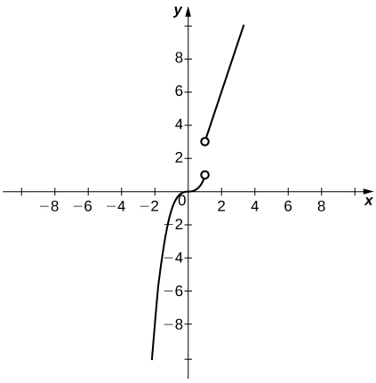
$A graph of the given piecewise function containing two segments. The first, x^3, exists for x < 1 and ends with an open circle at (1,1). The second, 3x, exists for x > 1. It beings with an open circle at (1,3).$

b. It is not possible to redefine $f(1)$ since the discontinuity is a jump discontinuity.

26) Let $f(x)=\dfrac{x^4−1}{x^2−1}$ for $x≠−1,1$.

a. Sketch the graph of $f$.

b. Is it possible to find values $k_1$ and $k_2$ such that $f(−1)=k$ and $f(1)=k_2$, and that makes $f(x)$ continuous for all real numbers? Briefly explain.

27) Sketch the graph of the function $y=f(x)$ with properties i. through vii.

i. The domain of $f$ is ($−∞,+∞$).

ii. $f$ has an infinite discontinuity at $x=−6$.

iii. $f(−6)=3$

iv. $\displaystyle \lim_{x→−3^−}f(x)=\lim_{x→−3^+}f(x)=2$

v. $f(−3)=3$

vi. $f$ is left continuous but not right continuous at $x=3$.

vii. $\displaystyle \lim_{x→−∞}f(x)=−∞$ and $\displaystyle \lim_{x→+∞}f(x)=+∞$

Answer

Answers may vary; see the following example:

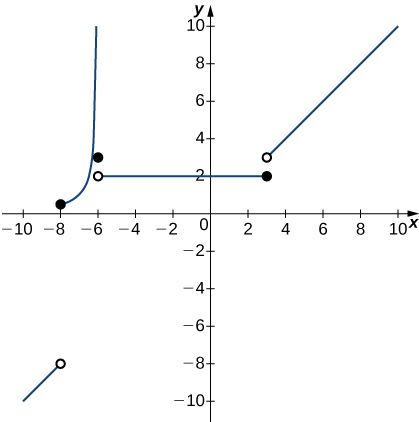
$A graph of a piecewise function with several segments. The first is an increasing line that exists for x < -8. It ends at an open circle at (-8,-8). The second is an increasing curve that exists from -8 <= x < -6. It begins with a closed circle at (-8, 0 ) and goes to infinity as x goes to -6 from the left. The third is a closed circle at the point (-6, 3). The fourth is a line that exists from -6 < x <= 3. It begins with an open circle at (-6, 2) and ends with a closed circle at (3,2). The fifth is an increasing line starting with an open circle at (3,3). It exists for x > 3.$

28) Sketch the graph of the function $y=f(x)$ with properties i. through iv.

i. The domain of $f$ is [$0,5$].

ii. $\displaystyle \lim_{x→1^+}f(x)$ and $\displaystyle \lim_{x→1^−}f(x)$ exist and are equal.

iii. $f(x)$ is left continuous but not continuous at $x=2$, and right continuous but not continuous at $x=3$.

iv. $f(x)$ has a removable discontinuity at $x=1$, a jump discontinuity at $x=2$, and the following limits hold: $\displaystyle \lim_{x→3^−}f(x)=−∞$ and $\displaystyle \lim_{x→3^+}f(x)=2$.

In exercises 29 - 30, suppose $y=f(x)$ is defined for all $x$. For each description, sketch a graph with the indicated property.

29) Discontinuous at $x=1$ with $\displaystyle \lim_{x→−1}f(x)=−1$ and $\displaystyle \lim_{x→2}f(x)=4$

Answer

Answers may vary; see the following example:

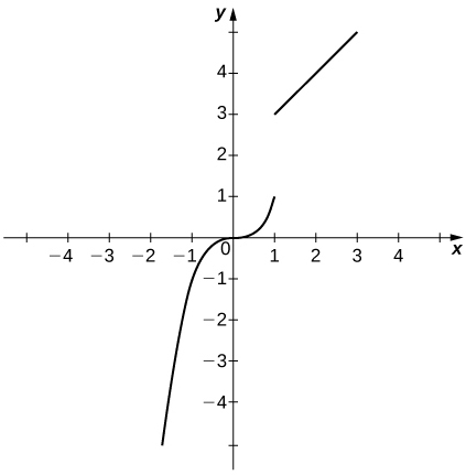
$The graph of a piecewise function with two parts. The first part is an increasing curve that exists for x < 1. It ends at (1,1). The second part is an increasing line that exists for x > 1. It begins at (1,3).$

30) Discontinuous at $x=2$ but continuous elsewhere with $\displaystyle \lim_{x→0}f(x)=\frac{1}{2}$

Determine whether each of the given statements is true. Justify your response with an explanation or counterexample.

31) $f(t)=\dfrac{2}{e^t−e^{−t}}$ is continuous everywhere.

Answer: False. It is continuous over ($−∞,0$) ∪ ($0,∞$).

32) If the left- and right-hand limits of $f(x)$ as $x→a$ exist and are equal, then $f$ cannot be discontinuous at $x=a$.

33) If a function is not continuous at a point, then it is not defined at that point.

Answer: False. Consider $f(x)=\begin{cases}x, & \text{if }x≠0\\ 4, & \text{if }x=0\end{cases}$.

34) According to the IVT, $\cos x−\sin x−x=2$ has a solution over the interval [$−1,1$].

35) If $f(x)$ is continuous such that $f(a)$ and $f(b)$ have opposite signs, then $f(x)=0$ has exactly one solution in [$a,b$].

Answer: False. Consider $f(x)=\cos(x)$ on [$−π,2π$].

36) The function $f(x)=\dfrac{x^2−4x+3}{x^2−1}$ is continuous over the interval [$0,3$].

37) If $f(x)$ is continuous everywhere and $f(a),f(b)>0$, then there is no root of $f(x)$ in the interval [$a,b$].

Answer: False. The IVT does not work in reverse! Consider $(x−1)^2$ over the interval [$−2,2$].

[T] The following problems consider the scalar form of Coulomb’s law, which describes the electrostatic force between two point charges, such as electrons. It is given by the equation $F(r)=k_e\dfrac{|q_1q_2|}{r^2}$, where $k_e$ is Coulomb’s constant, $q_i$ are the magnitudes of the charges of the two particles, and $r$ is the distance between the two particles.

38) To simplify the calculation of a model with many interacting particles, after some threshold value $r=R$, we approximate $F$ as zero.

a. Explain the physical reasoning behind this assumption.

b. What is the force equation?

c. Evaluate the force $F$ using both Coulomb’s law and our approximation, assuming two protons with a charge magnitude of $1.6022×10^{−19}$ coulombs (C), and the Coulomb constant $k_e=8.988×10^9Nm^2/C^2$ are 1 m apart. Also, assume $R<1$ m. How much inaccuracy does our approximation generate? Is our approximation reasonable?

d. Is there any finite value of R for which this system remains continuous at R?

39) Instead of making the force $0$ at $R$, we let the force be $10−20$ for $r≥R$. Assume two protons, which have a magnitude of charge $1.6022×10^{−19}\;C$, and the Coulomb constant $k_e=8.988×10^9\;Nm^2/C^2$. Is there a value $R$ that can make this system continuous? If so, find it.

Answer: $R=0.0001519$ m

Recall the discussion on spacecraft from the chapter opener. The following problems consider a rocket launch from Earth’s surface. The force of gravity on the rocket is given by $F(d)=−mk/d^2$, where m is the mass of the rocket, $d$ is the distance of the rocket from the center of Earth, and $k$ is a constant.

40) [T] Determine the value and units of $k$ given that the mass of the rocket on Earth is 3 million kg. (Hint: The distance from the center of Earth to its surface is 6378 km.)

41) [T] After a certain distance $D$ has passed, the gravitational effect of Earth becomes quite negligible, so we can approximate the force function by $F(d)=\begin{cases}−\dfrac{mk}{d^2}, & \text{if }d<D\\ 10,000, & \text{if }d≥D\end{cases}$. Find the necessary condition $D$ such that the force function remains continuous.

Answer: $D=63.78$ km

42) As the rocket travels away from Earth’s surface, there is a distance D where the rocket sheds some of its mass, since it no longer needs the excess fuel storage. We can write this function as $F(d)=\begin{cases} −\dfrac{m_1k}{d^2}, & \text{if }d<D \\ −\dfrac{m_2k}{d^2}, & \text{if }d≥D\end{cases}$. Is there a value of $D$ such that this function is continuous, assuming $m_1≠m_2$?

In Exercises 43 - 44, prove each function is continuous everywhere.

43) $f(θ)=\sin θ$

Answer: For all values of $a$, $f(a)$ is defined, $\displaystyle \lim_{θ→a}f(θ)$ exists, and $\displaystyle \lim_{θ→a}f(θ)=f(a)$. Therefore, $f(θ)$ is continuous everywhere.

44) $g(x)=|x|$

45) Where is $f(x)=\begin{cases} 0, & \text{if } x \text{ is irrational}\\ 1, & \text{if }x\text{ is rational}\end{cases}$ continuous?

Answer: Nowhere

2.5: The Precise Definition of a Limit

In exercises 1 - 4, write the appropriate $ ε − δ$ definition for each of the given statements.

1) $\displaystyle \lim_{x →a}f(x)=N$

2) $\displaystyle \lim_{t →b}g(t)=M$

Answer: For every $ ε >0$, there exists a $ δ >0$, so that if $0 <|t −b| < δ$, then $|g(t) −M| < ε$

3) $\displaystyle \lim_{x →c}h(x)=L$

4) $\displaystyle \lim_{x →a} φ(x)=A$

Answer: For every $ ε >0$, there exists a $ δ >0$, so that if $0 <|x −a| < δ$, then $| φ(x) −A| < ε$

The following graph of the function $f$ satisfies $\displaystyle \lim_{x →2}f(x)=2$. In the following exercises, determine a value of $ δ >0$ that satisfies each statement.

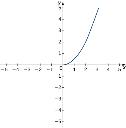
$A function drawn in quadrant one for x > 0. It is an increasing concave up function, with points approximately (0,0), (1, .5), (2,2), and (3,4).$

5) If $0 <|x −2| < δ$, then $|f(x) −2| <1$.

6) If $0 <|x −2| < δ$, then $|f(x) −2| <0.5$.

Answer: $ δ ≤0.25$

The following graph of the function $f$ satisfies $\displaystyle \lim_{x →3}f(x)= −1$. In the following exercises, determine a value of $ δ >0$ that satisfies each statement.

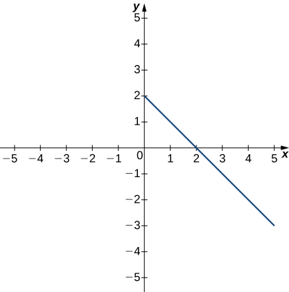
$A graph of a decreasing linear function, with points (0,2), (1,1), (2,0), (3,-1), (4,-2), and so on for x >= 0.$

7) If $0 <|x −3| < δ$, then $|f(x)+1| <1$.

8) If $0 <|x −3| < δ$, then $|f(x)+1| <2$.

Answer: $ δ ≤2$

The following graph of the function $f$ satisfies $\displaystyle \lim_{x →3}f(x)=2$. In the following exercises, for each value of $ ε$, find a value of $ δ >0$ such that the precise definition of limit holds true.

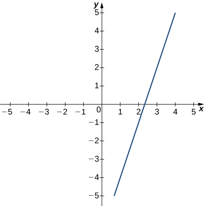
$A graph of an increasing linear function intersecting the x axis at about (2.25, 0) and going through the points (3,2) and, approximately, (1,-5) and (4,5).$

9) $ ε=1.5$

10) $ ε=3$

Answer: $ δ ≤1$

[T] In exercises 11 - 12, use a graphing calculator to find a number $ δ$ such that the statements hold true.

11) $\left|\sin(2x) −\frac{1}{2}\right| <0.1$, whenever $\left|x −\frac{ π}{12}\right| < δ$

12) $\left|\sqrt{x −4} −2\right| <0.1$, whenever $|x −8| < δ$

Answer: $ δ <0.3900$

In exercises 13 - 17, use the precise definition of limit to prove the given limits.

13) $\displaystyle \lim_{x →2}\,(5x+8)=18$

14) $\displaystyle \lim_{x →3}\frac{x^2 −9}{x −3}=6$

Answer: Let $ δ= ε$. If $0 <|x −3| < ε$, then $\left|\dfrac{x^2 −9}{x −3} - 6\right| = \left|\dfrac{(x+3)(x −3)}{x −3} - 6\right| = |x+3 −6|=|x −3| < ε$.

15) $\displaystyle \lim_{x →2}\frac{2x^2 −3x −2}{x −2}=5$

16) $\displaystyle \lim_{x →0}x^4=0$

Answer: Let $ δ=\sqrt[4]{ ε}$. If $0 <|x| <\sqrt[4]{ ε}$, then $\left|x^4-0\right|=x^4 < ε$.

17) $\displaystyle \lim_{x →2}\,(x^2+2x)=8$

In exercises 18 - 20, use the precise definition of limit to prove the given one-sided limits.

18) $\displaystyle \lim_{x →5^ −}\sqrt{5 −x}=0$

Answer: Let $ δ= ε^2$. If $- ε^2 < x - 5 < 0,$ we can multiply through by $-1$ to get $0 <5-x < ε^2.$
Then $\left|\sqrt{5 −x} - 0\right|=\sqrt{5 −x} < \sqrt{ ε^2} = ε$.

19) $\displaystyle \lim_{x →0^+}f(x)= −2$, where $f(x)=\begin{cases}8x −3, & \text{if }x <0\\4x −2, & \text{if }x ≥0\end{cases}$.

20) $\displaystyle \lim_{x →1^ −}f(x)=3$, where $f(x)=\begin{cases}5x −2, & \text{if }x <1\\7x −1, & \text{if }x ≥1\end{cases}$.

Answer: Let $ δ= ε/5$. If $ − ε/5 < x - 1 <0,$ we can multiply through by $-1$ to get $0 <1-x < ε/5.$
Then $|f(x) −3|=|5x-2-3| = |5x −5| = 5(1-x),$ since $x <1$ here.
And $5(1-x) < 5( ε/5) = ε$.

In exercises 21 - 23, use the precise definition of limit to prove the given infinite limits.

21) $\displaystyle \lim_{x →0}\frac{1}{x^2}= ∞$

22) $\displaystyle \lim_{x → −1}\frac{3}{(x+1)^2}= ∞$

Answer: Let $ δ=\sqrt{\frac{3}{N}}$. If $0 <|x+1| <\sqrt{\frac{3}{N}}$, then $f(x)=\frac{3}{(x+1)^2} >N$.

23) $\displaystyle \lim_{x →2} −\frac{1}{(x −2)^2}= − ∞$

24) An engineer is using a machine to cut a flat square of Aerogel of area $144 \,\text{cm}^2$. If there is a maximum error tolerance in the area of $8 \,\text{cm}^2$, how accurately must the engineer cut on the side, assuming all sides have the same length? How do these numbers relate to $ δ$, $ ε$, $a$, and $L$?

Answer: $0.033 \text{ cm}, \, ε=8,\, δ=0.33,\,a=12,\,L=144$

25) Use the precise definition of limit to prove that the following limit does not exist: $\displaystyle \lim_{x →1}\frac{|x −1|}{x −1}.$

26) Using precise definitions of limits, prove that $\displaystyle \lim_{x →0}f(x)$ does not exist, given that $f(x)$ is the ceiling function. (Hint: Try any $ δ <1$.)

Answer: Answers may very.

27) Using precise definitions of limits, prove that $\displaystyle \lim_{x →0}f(x)$ does not exist: $f(x)=\begin{cases}1, & \text{if }x\text{ is rational}\\0, & \text{if }x\text{ is irrational}\end{cases}$. (Hint: Think about how you can always choose a rational number $0 <d$, >

28) Using precise definitions of limits, determine $\displaystyle \lim_{x →0}f(x)$ for $f(x)=\begin{cases}x, & \text{if }x\text{ is rational}\\0, & \text{if }x\text{ is irrational}\end{cases}$. (Hint: Break into two cases, $x$ rational and $x$ irrational.)

Answer: $0$

29) Using the function from the previous exercise, use the precise definition of limits to show that $\displaystyle \lim_{x →a}f(x)$ does not exist for $a ≠0$

For exercises 30 - 32, suppose that $\displaystyle \lim_{x →a}f(x)=L$ and $\displaystyle \lim_{x →a}g(x)=M$ both exist. Use the precise definition of limits to prove the following limit laws:

30) $\displaystyle \lim_{x →a}(f(x) −g(x))=L −M$

Answer: $f(x) −g(x)=f(x)+( −1)g(x)$

31) $\displaystyle \lim_{x →a}[cf(x)]=cL$ for any real constant $c$ (Hint: Consider two cases: $c=0$ and $c ≠0$.)

32) $\displaystyle \lim_{x →a}[f(x)g(x)]=LM$. (Hint: $|f(x)g(x) −LM|= |f(x)g(x) −f(x)M +f(x)M −LM| ≤|f(x)||g(x) −M| +|M||f(x) −L|.)$

Answer: Answers may vary.

Chapter Review Exercises

True or False. In exercises 1 - 4, justify your answer with a proof or a counterexample.

1) A function has to be continuous at $x=a$ if the $\displaystyle \lim_{x→a}f(x)$ exists.

2) You can use the quotient rule to evaluate $\displaystyle \lim_{x→0}\frac{\sin x}{x}$.

Answer: False, since we cannot have $\displaystyle \lim_{x→0}x=0$ in the denominator.

3) If there is a vertical asymptote at $x=a$ for the function $f(x)$, then $f$ is undefined at the point $x=a$.

4) If $\displaystyle \lim_{x→a}f(x)$ does not exist, then $f$ is undefined at the point $x=a$.

Answer: False. A jump discontinuity is possible.

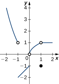
5) Using the graph, find each limit or explain why the limit does not exist.

a. $\displaystyle \lim_{x→−1}f(x)$

b. $\displaystyle \lim_{x→1}f(x)$

c. $\displaystyle \lim_{x→0^+}f(x)$

d. $\displaystyle \lim_{x→2}f(x)$

$A graph of a piecewise function with several segments. The first is a decreasing concave up curve existing for x < -1. It ends at an open circle at (-1, 1). The second is an increasing linear function starting at (-1, -2) and ending at (0,-1). The third is an increasing concave down curve existing from an open circle at (0,0) to an open circle at (1,1). The fourth is a closed circle at (1,-1). The fifth is a line with no slope existing for x > 1, starting at the open circle at (1,1).$

In exercises 6 - 15, evaluate the limit algebraically or explain why the limit does not exist.

6) $\displaystyle \lim_{x→2}\frac{2x^2−3x−2}{x−2}$

Answer: $5$

7) $\displaystyle \lim_{x→0}3x^2−2x+4$

8) $\displaystyle \lim_{x→3}\frac{x^3−2x^2−1}{3x−2}$

Answer: $8/7$

9) $\displaystyle \lim_{x→π/2}\frac{\cot x}{\cos x}$

10) $\displaystyle \lim_{x→−5}\frac{x^2+25}{x+5}$

Answer: DNE

11) $\displaystyle \lim_{x→2}\frac{3x^2−2x−8}{x^2−4}$

12) $\displaystyle \lim_{x→1}\frac{x^2−1}{x^3−1}$

Answer: $2/3$

13) $\displaystyle \lim_{x→1}\frac{x^2−1}{\sqrt{x}−1}$

14) $\displaystyle \lim_{x→4}\frac{4−x}{\sqrt{x}−2}$

Answer: $−4$

15) $\displaystyle \lim_{x→4}\frac{1}{\sqrt{x}−2}$

In exercises 16 - 17, use the squeeze theorem to prove the limit.

16) $\displaystyle \lim_{x→0}x^2\cos(2πx)=0$

Answer: Since $−1≤\cos(2πx)≤1$, then $−x^2≤x^2\cos(2πx)≤x^2$. Since $\displaystyle \lim_{x→0}x^2=0=\lim_{x→0}−x^2$, it follows that $\displaystyle \lim_{x→0}x^2\cos(2πx)=0$.

17) $\displaystyle \lim_{x→0}x^3\sin\left(\frac{π}{x}\right)=0$

18) Determine the domain such that the function $f(x)=\sqrt{x−2}+xe^x$ is continuous over its domain.

Answer: $[2,∞]$

In exercises 19 - 20, determine the value of $c$ such that the function remains continuous. Draw your resulting function to ensure it is continuous.

19) $f(x)=\begin{cases}x^2+1, & \text{if } x>c\\2^x, & \text{if } x≤c\end{cases}$

20) $f(x)=\begin{cases}\sqrt{x+1}, & \text{if } x>−1\\x^2+c, & \text{if } x≤−1\end{cases}$

In exercises 21 - 22, use the precise definition of limit to prove the limit.

21) $\displaystyle \lim_{x→1}\,(8x+16)=24$

22) $\displaystyle \lim_{x→0}x^3=0$

Answer: $δ=\sqrt[3]{ε}$

23) A ball is thrown into the air and the vertical position is given by $x(t)=−4.9t^2+25t+5$. Use the Intermediate Value Theorem to show that the ball must land on the ground sometime between 5 sec and 6 sec after the throw.

24) A particle moving along a line has a displacement according to the function $x(t)=t^2−2t+4$, where $x$ is measured in meters and $t$ is measured in seconds. Find the average velocity over the time period $t=[0,2]$.

Answer: $0$ m/sec

25) From the previous exercises, estimate the instantaneous velocity at $t=2$ by checking the average velocity within $t=0.01$ sec.

Search

Text Color

Text Size

Margin Size

Font Type

Intuitive Definition of Limits

Infinite Limits

\(x\)	\(y\)	\(Q(x,y)\)	\(m_{sec}\)
1.1	a.	e.	i.
1.01	b.	f.	j.
1.001	c.	g.	k.
1.0001	d.	h.	l.

\(x\)	\(y\)	\(Q(x,y)\)	\(m_{sec}\)
4.1	a.	e.	i.
4.01	b.	f.	j.
4.001	c.	g.	k.
4.0001	d.	h.	l.

\(x\)	\(y\)	\(Q(ϕ,y)\)	\(m_{sec}\)
1.4	a.	e.	i.
1.49	b.	f.	j.
1.499	c.	g.	k.
1.4999	d.	h.	l.

\(x\)	\(y\)	\(Q(x,y)\)	\(m_{sec}\)
-1.05	a.	e.	i.
-1.01	b.	f.	j.
-1.005	c.	g.	k.
-1.001	d.	h.	l.