
4.9: Antiderivatives
- Page ID
- 4469
\( \newcommand{\vecs}[1]{\overset { \scriptstyle \rightharpoonup} {\mathbf{#1}} } \)
\( \newcommand{\vecd}[1]{\overset{-\!-\!\rightharpoonup}{\vphantom{a}\smash {#1}}} \)
\( \newcommand{\dsum}{\displaystyle\sum\limits} \)
\( \newcommand{\dint}{\displaystyle\int\limits} \)
\( \newcommand{\dlim}{\displaystyle\lim\limits} \)
\( \newcommand{\id}{\mathrm{id}}\) \( \newcommand{\Span}{\mathrm{span}}\)
( \newcommand{\kernel}{\mathrm{null}\,}\) \( \newcommand{\range}{\mathrm{range}\,}\)
\( \newcommand{\RealPart}{\mathrm{Re}}\) \( \newcommand{\ImaginaryPart}{\mathrm{Im}}\)
\( \newcommand{\Argument}{\mathrm{Arg}}\) \( \newcommand{\norm}[1]{\| #1 \|}\)
\( \newcommand{\inner}[2]{\langle #1, #2 \rangle}\)
\( \newcommand{\Span}{\mathrm{span}}\)
\( \newcommand{\id}{\mathrm{id}}\)
\( \newcommand{\Span}{\mathrm{span}}\)
\( \newcommand{\kernel}{\mathrm{null}\,}\)
\( \newcommand{\range}{\mathrm{range}\,}\)
\( \newcommand{\RealPart}{\mathrm{Re}}\)
\( \newcommand{\ImaginaryPart}{\mathrm{Im}}\)
\( \newcommand{\Argument}{\mathrm{Arg}}\)
\( \newcommand{\norm}[1]{\| #1 \|}\)
\( \newcommand{\inner}[2]{\langle #1, #2 \rangle}\)
\( \newcommand{\Span}{\mathrm{span}}\) \( \newcommand{\AA}{\unicode[.8,0]{x212B}}\)
\( \newcommand{\vectorA}[1]{\vec{#1}} % arrow\)
\( \newcommand{\vectorAt}[1]{\vec{\text{#1}}} % arrow\)
\( \newcommand{\vectorB}[1]{\overset { \scriptstyle \rightharpoonup} {\mathbf{#1}} } \)
\( \newcommand{\vectorC}[1]{\textbf{#1}} \)
\( \newcommand{\vectorD}[1]{\overrightarrow{#1}} \)
\( \newcommand{\vectorDt}[1]{\overrightarrow{\text{#1}}} \)
\( \newcommand{\vectE}[1]{\overset{-\!-\!\rightharpoonup}{\vphantom{a}\smash{\mathbf {#1}}}} \)
\( \newcommand{\vecs}[1]{\overset { \scriptstyle \rightharpoonup} {\mathbf{#1}} } \)
\(\newcommand{\longvect}{\overrightarrow}\)
\( \newcommand{\vecd}[1]{\overset{-\!-\!\rightharpoonup}{\vphantom{a}\smash {#1}}} \)
\(\newcommand{\avec}{\mathbf a}\) \(\newcommand{\bvec}{\mathbf b}\) \(\newcommand{\cvec}{\mathbf c}\) \(\newcommand{\dvec}{\mathbf d}\) \(\newcommand{\dtil}{\widetilde{\mathbf d}}\) \(\newcommand{\evec}{\mathbf e}\) \(\newcommand{\fvec}{\mathbf f}\) \(\newcommand{\nvec}{\mathbf n}\) \(\newcommand{\pvec}{\mathbf p}\) \(\newcommand{\qvec}{\mathbf q}\) \(\newcommand{\svec}{\mathbf s}\) \(\newcommand{\tvec}{\mathbf t}\) \(\newcommand{\uvec}{\mathbf u}\) \(\newcommand{\vvec}{\mathbf v}\) \(\newcommand{\wvec}{\mathbf w}\) \(\newcommand{\xvec}{\mathbf x}\) \(\newcommand{\yvec}{\mathbf y}\) \(\newcommand{\zvec}{\mathbf z}\) \(\newcommand{\rvec}{\mathbf r}\) \(\newcommand{\mvec}{\mathbf m}\) \(\newcommand{\zerovec}{\mathbf 0}\) \(\newcommand{\onevec}{\mathbf 1}\) \(\newcommand{\real}{\mathbb R}\) \(\newcommand{\twovec}[2]{\left[\begin{array}{r}#1 \\ #2 \end{array}\right]}\) \(\newcommand{\ctwovec}[2]{\left[\begin{array}{c}#1 \\ #2 \end{array}\right]}\) \(\newcommand{\threevec}[3]{\left[\begin{array}{r}#1 \\ #2 \\ #3 \end{array}\right]}\) \(\newcommand{\cthreevec}[3]{\left[\begin{array}{c}#1 \\ #2 \\ #3 \end{array}\right]}\) \(\newcommand{\fourvec}[4]{\left[\begin{array}{r}#1 \\ #2 \\ #3 \\ #4 \end{array}\right]}\) \(\newcommand{\cfourvec}[4]{\left[\begin{array}{c}#1 \\ #2 \\ #3 \\ #4 \end{array}\right]}\) \(\newcommand{\fivevec}[5]{\left[\begin{array}{r}#1 \\ #2 \\ #3 \\ #4 \\ #5 \\ \end{array}\right]}\) \(\newcommand{\cfivevec}[5]{\left[\begin{array}{c}#1 \\ #2 \\ #3 \\ #4 \\ #5 \\ \end{array}\right]}\) \(\newcommand{\mattwo}[4]{\left[\begin{array}{rr}#1 \amp #2 \\ #3 \amp #4 \\ \end{array}\right]}\) \(\newcommand{\laspan}[1]{\text{Span}\{#1\}}\) \(\newcommand{\bcal}{\cal B}\) \(\newcommand{\ccal}{\cal C}\) \(\newcommand{\scal}{\cal S}\) \(\newcommand{\wcal}{\cal W}\) \(\newcommand{\ecal}{\cal E}\) \(\newcommand{\coords}[2]{\left\{#1\right\}_{#2}}\) \(\newcommand{\gray}[1]{\color{gray}{#1}}\) \(\newcommand{\lgray}[1]{\color{lightgray}{#1}}\) \(\newcommand{\rank}{\operatorname{rank}}\) \(\newcommand{\row}{\text{Row}}\) \(\newcommand{\col}{\text{Col}}\) \(\renewcommand{\row}{\text{Row}}\) \(\newcommand{\nul}{\text{Nul}}\) \(\newcommand{\var}{\text{Var}}\) \(\newcommand{\corr}{\text{corr}}\) \(\newcommand{\len}[1]{\left|#1\right|}\) \(\newcommand{\bbar}{\overline{\bvec}}\) \(\newcommand{\bhat}{\widehat{\bvec}}\) \(\newcommand{\bperp}{\bvec^\perp}\) \(\newcommand{\xhat}{\widehat{\xvec}}\) \(\newcommand{\vhat}{\widehat{\vvec}}\) \(\newcommand{\uhat}{\widehat{\uvec}}\) \(\newcommand{\what}{\widehat{\wvec}}\) \(\newcommand{\Sighat}{\widehat{\Sigma}}\) \(\newcommand{\lt}{<}\) \(\newcommand{\gt}{>}\) \(\newcommand{\amp}{&}\) \(\definecolor{fillinmathshade}{gray}{0.9}\)At this point, we have seen how to calculate derivatives of many functions and have been introduced to a variety of their applications. We now ask a question that turns this process around: Given a function \(f\), how do we find a function with the derivative \(f\) and why would we be interested in such a function?
We answer the first part of this question by defining antiderivatives. The antiderivative of a function \(f\) is a function with a derivative \(f\). Why are we interested in antiderivatives? The need for antiderivatives arises in many situations, and we look at various examples throughout the remainder of the text. Here we examine one specific example that involves rectilinear motion. In our examination in Derivatives of rectilinear motion, we showed that given a position function \(s(t)\) of an object, then its velocity function \(v(t)\) is the derivative of \(s(t)\)—that is, \(v(t)=s′(t)\). Furthermore, the acceleration \(a(t)\) is the derivative of the velocity \(v(t)\)—that is, \(a(t)=v′(t)=s''(t)\). Now suppose we are given an acceleration function \(a\), but not the velocity function v or the position function \(s\). Since \(a(t)=v′(t)\), determining the velocity function requires us to find an antiderivative of the acceleration function. Then, since \(v(t)=s′(t),\) determining the position function requires us to find an antiderivative of the velocity function. Rectilinear motion is just one case in which the need for antiderivatives arises. We will see many more examples throughout the remainder of the text. For now, let’s look at the terminology and notation for antiderivatives, and determine the antiderivatives for several types of functions. We examine various techniques for finding antiderivatives of more complicated functions later in the text (Introduction to Techniques of Integration).
The Reverse of Differentiation
At this point, we know how to find derivatives of various functions. We now ask the opposite question. Given a function \(f\), how can we find a function with derivative \(f\)? If we can find a function \(F\) derivative \(f,\) we call \(F\) an antiderivative of \(f\).
Definition: Antiderivative
A function \(F\) is an antiderivative of the function \(f\) if
\[F′(x)=f(x)\]
for all \(x\) in the domain of \(f\).
Consider the function \(f(x)=2x\). Knowing the power rule of differentiation, we conclude that \(F(x)=x^2\) is an antiderivative of \(f\) since \(F′(x)=2x\). Are there any other antiderivatives of \(f\)? Yes; since the derivative of any constant \(C\) is zero, \(x^2+C\) is also an antiderivative of \(2x\). Therefore, \(x^2+5\) and \(x^2−\sqrt{2}\) are also antiderivatives. Are there any others that are not of the form \(x^2+C\) for some constant \(C\)? The answer is no. From Corollary 2 of the Mean Value Theorem, we know that if \(F\) and \(G\) are differentiable functions such that \(F′(x)=G′(x),\) then \(F(x)−G(x)=C\) for some constant \(C\). This fact leads to the following important theorem.
General Form of an Antiderivative
Let \(F\) be an antiderivative of \(f\) over an interval \(I\). Then,
- for each constant \(C\), the function \(F(x)+C\) is also an antiderivative of \(f\) over \(I\);
- if \(G\) is an antiderivative of \(f\) over \(I\), there is a constant \(C\) for which \(G(x)=F(x)+C\) over \(I\).
In other words, the most general form of the antiderivative of \(f\) over \(I\) is \(F(x)+C\).
We use this fact and our knowledge of derivatives to find all the antiderivatives for several functions.
Example \(\PageIndex{1}\): Finding Antiderivatives
For each of the following functions, find all antiderivatives.
- \(f(x)=3x^2\)
- \(f(x)=\dfrac{1}{x}\)
- \(f(x)=\cos x\)
- \(f(x)=e^x\)
Solution:
a. Because
\[\dfrac{d}{dx}(x^3)=3x^2 \nonumber\]
then \(F(x)=x^3\) is an antiderivative of \(3x^2\). Therefore, every antiderivative of \(3x^2\) is of the form \(x^3+C\) for some constant \(C\), and every function of the form \(x^3+C\) is an antiderivative of \(3x^2\).
b. Let \(f(x)=\ln |x|.\) For \(x>0,f(x)=\ln (x)\) and
\[\dfrac{d}{dx}(\ln x)=\dfrac{1}{x}. \nonumber\]
For\( x<0,f(x)=\ln (−x)\) and
\[\dfrac{d}{dx}(\ln (−x))=−\dfrac{1}{−x}=\dfrac{1}{x}. \nonumber\]
Therefore,
\[\dfrac{d}{dx}(\ln |x|)=\dfrac{1}{x}. \nonumber\]
Thus, \(F(x)=\ln |x|\) is an antiderivative of \(\dfrac{1}{x}\). Therefore, every antiderivative of \(\dfrac{1}{x}\) is of the form \(\ln |x|+C\) for some constant \(C\) and every function of the form \(\ln |x|+C\) is an antiderivative of \(\dfrac{1}{x}\).
c. We have
\[\dfrac{d}{dx}(\sin x)=\cos x, \nonumber\]
so \(F(x)=\sin x\) is an antiderivative of \(\cos x\). Therefore, every antiderivative of \(\cos x\) is of the form \(\sin x+C\) for some constant \(C\) and every function of the form \(\sin x+C\) is an antiderivative of \(\cos x\).
d. Since
\[\dfrac{d}{dx}(e^x)=e^x, \nonumber\]
then \(F(x)=e^x\) is an antiderivative of \(e^x\). Therefore, every antiderivative of \(e^x\) is of the form \(e^x+C\) for some constant \(C\) and every function of the form \(e^x+C\) is an antiderivative of \(e^x\).
Exercise \(\PageIndex{1}\)
Find all antiderivatives of \(f(x)=\sin x\).
- Hint
-
What function has a derivative of \(\sin x\)?
- Answer
-
\(−\cos x+C\)
Indefinite Integrals
We now look at the formal notation used to represent antiderivatives and examine some of their properties. These properties allow us to find antiderivatives of more complicated functions. Given a function \(f\), we use the notation \(f′(x)\) or \(\dfrac{df}{dx}\) to denote the derivative of \(f\). Here we introduce notation for antiderivatives. If \(F\) is an antiderivative of \(f\), we say that \(F(x)+C\) is the most general antiderivative of \(f\) and write
\[\int f(x)dx=F(x)+C.\]
The symbol \(\int \) is called an integral sign, and \(\int f(x)dx\) is called the indefinite integral of \(f\).
Definition: Indefinite Integrals
Given a function \(f\), the indefinite integral of \(f\), denoted
\[\int f(x)dx,\]
is the most general antiderivative of \(f\). If \(F\) is an antiderivative of \(f\), then
\[\int f(x)dx=F(x)+C.\]
The expression \(f(x)\) is called the integrand and the variable x is the variable of integration.
Given the terminology introduced in this definition, the act of finding the antiderivatives of a function \(f\) is usually referred to as integrating \(f\).
For a function \(f\) and an antiderivative \(F\), the functions \(F(x)+C\), where \(C\) is any real number, is often referred to as the family of antiderivatives of \(f\). For example, since \(x^2\) is an antiderivative of \(2x\) and any antiderivative of \(2x\) is of the form \(x^2+C,\) we write
\[\int 2xdx=x^2+C.\]
The collection of all functions of the form \(x^2+C,\) where \(C\) is any real number, is known as the family of antiderivatives of \(2x\). Figure shows a graph of this family of antiderivatives.
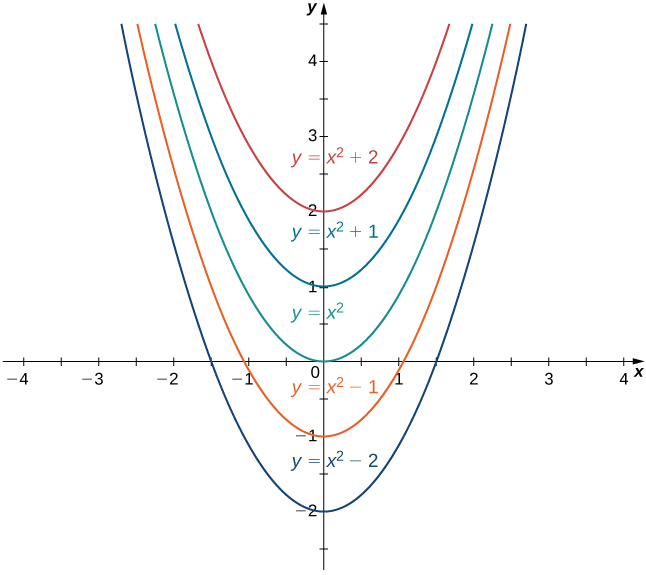
Figure \(\PageIndex{1}\): The family of antiderivatives of \(2x\) consists of all functions of the form \(x^2+C\), where \(C\) is any real number.
For some functions, evaluating indefinite integrals follows directly from properties of derivatives. For example, for \(n≠−1\),
\(\int x^ndx=\dfrac{x^{n+1}}{n+1}+C,\)
which comes directly from
\(\dfrac{d}{dx}(\dfrac{x^{n+1}}{n+1})=(n+1)\dfrac{x^n}{n+1}=x^n\).
This fact is known as the power rule for integrals.
Power Rule for Integrals
For \(n≠−1,\)
\[\int x^ndx=\dfrac{x^{n+1}}{n+1}+C.\]
Evaluating indefinite integrals for some other functions is also a straightforward calculation. The following table lists the indefinite integrals for several common functions. A more complete list appears in Appendix B.
| Differentiation Formula | Indefinite Integral |
|---|---|
| \(\dfrac{d}{dx}(k)=0\) | \(\int kdx=\int kx^0dx=kx+C\) |
| \(\dfrac{d}{dx}(x^n)=nx^{n−1}\) | \(\int x^ndn=\dfrac{x^{n+1}}{n+1}+C\) for \(n≠−1\) |
| \(\dfrac{d}{dx}(\ln |x|)=\dfrac{1}{x}\) | \(\int \dfrac{1}{x}dx=\ln |x|+C\) |
| \(\dfrac{d}{dx}(e^x)=e^x\) | \(\int e^xdx=e^x+C\) |
| \(\dfrac{d}{dx}(\sin x)=\cos x\) | \(\int \cos xdx=\sin x+C\) |
| \(\dfrac{d}{dx}(\cos x)=−\sin x\) | \(\int \sin xdx=−\cos x+C\) |
| \(\dfrac{d}{dx}(\tan x)=sec^2x\) | \(\int sec^2xdx=\tan x+C\) |
| \(\dfrac{d}{dx}(cscx)=−cscx\cot x\) | \(\int cscx\cot xdx=−cscx+C\) |
| \(\dfrac{d}{dx}(secx)=secx\tan x\) | \(\int secx\tan xdx=secx+C\) |
| \(\dfrac{d}{dx}(\cot x)=−csc^2x\) | \(\int csc^2xdx=−\cot x+C\) |
| \(\dfrac{d}{dx}(sin^{−1}x)=\dfrac{1}{\sqrt{1−x^2}}\) | \(\int \dfrac{1}{\sqrt{1−x^2}}=sin^{−1}x+C\) |
| \(\dfrac{d}{dx}(tan^{−1}x)=\dfrac{1}{1+x^2}\) | \(\int \dfrac{1}{1+x^2}dx=tan^{−1}x+C\) |
| \(\dfrac{d}{dx}(sec^{−1}|x|)=\dfrac{1}{x\sqrt{x^2−1}}\) | \(\int \dfrac{1}{x\sqrt{x^2−1}}dx=sec^{−1}|x|+C\) |
From the definition of indefinite integral of \(f\), we know
\[\int f(x)dx=F(x)+C\]
if and only if \(F\) is an antiderivative of \(f\). Therefore, when claiming that
\[\int f(x)dx=F(x)+C\]
it is important to check whether this statement is correct by verifying that \(F′(x)=f(x).\)
Example \(\PageIndex{2}\): Verifying an Indefinite Integral
Each of the following statements is of the form \(\int f(x)dx=F(x)+C.\) Verify that each statement is correct by showing that \(F′(x)=f(x).\)
- \(\int (x+e^x)dx=\dfrac{x^2}{2}+e^x+C\)
- \(\int xe^xdx=xe^x−e^x+C\)
Solution:
a. Since
\(\dfrac{d}{dx}(\dfrac{x^2}{2}+e^x+C)=x+e^x\),
the statement
\[\int (x+e^x)dx=\dfrac{x^2}{2}+e^x+C \nonumber\]
is correct.
Note that we are verifying an indefinite integral for a sum. Furthermore, \(\dfrac{x^2}{2}\) and \(e^x\) are antiderivatives of \(x\) and \(e^x\), respectively, and the sum of the antiderivatives is an antiderivative of the sum. We discuss this fact again later in this section.
b. Using the product rule, we see that
\[\dfrac{d}{dx}(xe^x−e^x+C)=e^x+xe^x−e^x=xe^x. \nonumber\]
Therefore, the statement
\[\int xe^xdx=xe^x−e^x+C \nonumber\]
is correct.
Note that we are verifying an indefinite integral for a product. The antiderivative xex−ex is not a product of the antiderivatives. Furthermore, the product of antiderivatives, \(x^2e^x/2\) is not an antiderivative of \(xe^x\) since
\(\dfrac{d}{dx}(\dfrac{x^2e^x}{2})=xe^x+\dfrac{x^2e^x}{2}≠xe^x\).
In general, the product of antiderivatives is not an antiderivative of a product.
Exercise \(\PageIndex{2}\)
Verify that \[\int x\cos x\,dx=x\sin x+\cos x+C.\nonumber\]
- Hint
-
Calculate \[\dfrac{d}{dx}(x\sin x+\cos x+C).\nonumber\]
- Answer
-
\[\dfrac{d}{dx}(x\sin x+\cos x+C)=\sin x+x\cos x−\sin x=x \cos x\nonumber\]
In Table, we listed the indefinite integrals for many elementary functions. Let’s now turn our attention to evaluating indefinite integrals for more complicated functions. For example, consider finding an antiderivative of a sum \(f+g\). In Example a. we showed that an antiderivative of the sum \(x+e^x\) is given by the sum (\(\dfrac{x^2}{2})+e^x\)—that is, an antiderivative of a sum is given by a sum of antiderivatives. This result was not specific to this example. In general, if \(F\) and \(G\) are antiderivatives of any functions \(f\) and \(g\), respectively, then
\(\dfrac{d}{dx}(F(x)+G(x))=F′(x)+G′(x)=f(x)+g(x).\)
Therefore, \(F(x)+G(x)\) is an antiderivative of \(f(x)+g(x)\) and we have
\[ \int (f(x)+g(x))dx=F(x)+G(x)+C.\nonumber\]
Similarly,
\[ \int (f(x)−g(x))dx=F(x)−G(x)+C.\nonumber\]
In addition, consider the task of finding an antiderivative of \(kf(x),\) where \(k\) is any real number. Since
\[ \dfrac{d}{dx}(kf(x))=k\dfrac{d}{dx}F(x)=kF′(x)\nonumber\]
for any real number \(k\), we conclude that
\[ \int kf(x)dx=kF(x)+C.\nonumber\]
These properties are summarized next.
Properties of Indefinite Integrals
Let \(F\) and \(G\) be antiderivatives of \(f\) and \(g\), respectively, and let \(k\) be any real number.
Sums and Differences
\(\int (f(x)±g(x))dx=F(x)±G(x)+C\)
Constant Multiples
\(\int kf(x)dx=kF(x)+C\)
From this theorem, we can evaluate any integral involving a sum, difference, or constant multiple of functions with antiderivatives that are known. Evaluating integrals involving products, quotients, or compositions is more complicated (see Exampleb. for an example involving an antiderivative of a product.) We look at and address integrals involving these more complicated functions in Introduction to Integration. In the next example, we examine how to use this theorem to calculate the indefinite integrals of several functions.
Example \(\PageIndex{3}\): Evaluating Indefinite Integrals
Evaluate each of the following indefinite integrals:
- \(\int (5x^3−7x^2+3x+4)dx\)
- \(\int \dfrac{x^2+4\sqrt[3]{x}}{x}dx\)
- \(\int \dfrac{4}{1+x^2}dx\)
- \(\int \tan x\cos xdx\)
Solution:
a. Using Note, we can integrate each of the four terms in the integrand separately. We obtain
\(\int (5x^3−7x^2+3x+4)dx=\int 5x^3dx−\int 7x^2dx+\int 3xdx+\int 4dx.\)
From the second part of Note, each coefficient can be written in front of the integral sign, which gives
\(\int 5x^3dx−\int 7x^2dx+\int 3xdx+\int 4dx=5\int x^3dx−7\int x^2dx+3\int xdx+4\int 1dx.\)
Using the power rule for integrals, we conclude that
\(\int (5x^3−7x^2+3x+4)dx=\dfrac{5}{4}x^4−\dfrac{7}{3}x^3+\dfrac{3}{2}x^2+4x+C.\)
b. Rewrite the integrand as
\(\dfrac{x^2+4\sqrt[3]{x}}{x}=\dfrac{x^2}{x}+\dfrac{4\sqrt[3]{x}}{x}=0.\)
Then, to evaluate the integral, integrate each of these terms separately. Using the power rule, we have
\(\int (x+\dfrac{4}{x^{2/3}})dx=\int xdx+4\int x^{−2/3}dx\)
\(=\dfrac{1}{2}x^2+4\dfrac{1}{(\dfrac{−2}{3})+1}x^{(−2/3)+1}+C])\)
\(=\dfrac{1}{2}x^2+12x^{1/3}+C.\)
c. Using Note, write the integral as
\(4\int \dfrac{1}{1+x^2}dx.\)
Then, use the fact that \(tan^{−1}(x)\) is an antiderivative of \(\dfrac{1}{(1+x^2)}\) to conclude that
\(\int \dfrac{4}{1+x^2}dx=4tan^{−1}(x)+C.\)
d. Rewrite the integrand as
\(\tan x\cos x=\dfrac{\sin x}{\cos x}\cos x=\sin x.\)
Therefore,
\(\int \tan x\cos x=\int \sin x=−\cos x+C.\)
Exercise \(\PageIndex{3}\)
Evaluate \(\int (4x^3−5x^2+x−7)dx\).
- Hint
-
Integrate each term in the integrand separately, making use of the power rule.
- Answer
-
\(x^4−\dfrac{5}{3}x^3+\dfrac{1}{2}x^2−7x+C\)
Initial-Value Problems
We look at techniques for integrating a large variety of functions involving products, quotients, and compositions later in the text. Here we turn to one common use for antiderivatives that arises often in many applications: solving differential equations.
A differential equation is an equation that relates an unknown function and one or more of its derivatives. The equation
is a simple example of a differential equation. Solving this equation means finding a function \(y\) with a derivative \(f\). Therefore, the solutions of Equation are the antiderivatives of \(f\). If \(F\) is one antiderivative of \( f\), every function of the form \( y=F(x)+C\) is a solution of that differential equation. For example, the solutions of
are given by
Sometimes we are interested in determining whether a particular solution curve passes through a certain point \( (x_0,y_0)\) —that is, \( y(x_0)=y_0\). The problem of finding a function \(y\) that satisfies a differential equation
with the additional condition
is an example of an initial-value problem. The condition \( y(x_0)=y_0\) is known as an initial condition. For example, looking for a function \( y\) that satisfies the differential equation
and the initial condition
is an example of an initial-value problem. Since the solutions of the differential equation are \( y=2x^3+C,\) to find a function \(y\) that also satisfies the initial condition, we need to find \(C\) such that \(y(1)=2(1)^3+C=5\). From this equation, we see that \( C=3\), and we conclude that \( y=2x^3+3\) is the solution of this initial-value problem as shown in the following graph.
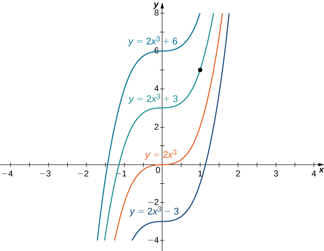
Figure \(\PageIndex{2}\): Some of the solution curves of the differential equation \(\dfrac{dy}{dx}=6x^2\) are displayed. The function \(y=2x^3+3\) satisfies the differential equation and the initial condition \(y(1)=5.\)
Example \(\PageIndex{4}\): Solving an Initial-Value Problem
Solve the initial-value problem
\[\dfrac{dy}{dx}=\sin x,y(0)=5.\]
Solution
First we need to solve the differential equation. If \(\dfrac{dy}{dx}=\sin x\), then
\[y=\int sin(x)dx=−\cos x+C.\]
Next we need to look for a solution \(y\) that satisfies the initial condition. The initial condition y(0)=5 means we need a constant \(C\) such that \(−\cos x+C=5.\) Therefore,
\[C=5+cos(0)=6.\]
The solution of the initial-value problem is \(y=−\cos x+6.\)
Exercise \(\PageIndex{4}\)
Solve the initial value problem \(\dfrac{dy}{dx}=3x^{−2},y(1)=2\).
- Hint
-
Find all antiderivatives of \(f(x)=3x^{−2.}\)
- Answer
-
\(y=−\dfrac{3}{x}+5\)
Initial-value problems arise in many applications. Next we consider a problem in which a driver applies the brakes in a car. We are interested in how long it takes for the car to stop. Recall that the velocity function \(v(t)\) is the derivative of a position function \(s(t),\) and the acceleration \(a(t)\) is the derivative of the velocity function. In earlier examples in the text, we could calculate the velocity from the position and then compute the acceleration from the velocity. In the next example we work the other way around. Given an acceleration function, we calculate the velocity function. We then use the velocity function to determine the position function.
Example \(\PageIndex{5}\):
A car is traveling at the rate of \(88\) ft/sec (\(60\) mph) when the brakes are applied. The car begins decelerating at a constant rate of \(15\) ft/sec2.
- How many seconds elapse before the car stops?
- How far does the car travel during that time?
Solution
a. First we introduce variables for this problem. Let \(t\) be the time (in seconds) after the brakes are first applied. Let \(a(t)\) be the acceleration of the car (in feet per seconds squared) at time \(t\). Let \(v(t)\) be the velocity of the car (in feet per second) at time \(t\). Let \(s(t)\) be the car’s position (in feet) beyond the point where the brakes are applied at time \(t\).
The car is traveling at a rate of \(88ft/sec\). Therefore, the initial velocity is \(v(0)=88\) ft/sec. Since the car is decelerating, the acceleration is
\(a(t)=−15ft/s^2\).
The acceleration is the derivative of the velocity,
\(v′(t)=15.\)
Therefore, we have an initial-value problem to solve:
\(v′(t)=−15,v(0)=88.\)
Integrating, we find that
\(v(t)=−15t+C.\)
Since \(v(0)=88,C=88.\) Thus, the velocity function is
\(v(t)=−15t+88.\)
To find how long it takes for the car to stop, we need to find the time t such that the velocity is zero. Solving \(−15t+88=0,\) we obtain \(t=\dfrac{88}{15}\) sec.
b. To find how far the car travels during this time, we need to find the position of the car after \(\dfrac{88}{15}\) sec. We know the velocity \(v(t)\) is the derivative of the position \(s(t)\). Consider the initial position to be \(s(0)=0\). Therefore, we need to solve the initial-value problem
\(s′(t)=−15t+88,s(0)=0.\)
Integrating, we have
\(s(t)=−\dfrac{15}{2}t^2+88t+C.\)
Since \(s(0)=0\), the constant is \(C=0\). Therefore, the position function is
\(s(t)=−\dfrac{15}{2}t^2+88t.\)
After \(t=\dfrac{88}{15}\) sec, the position is \(s(\dfrac{88}{15})≈258.133\) ft.
Exercise \(\PageIndex{5}\)
Suppose the car is traveling at the rate of \(44\) ft/sec. How long does it take for the car to stop? How far will the car travel?
- Hint
-
\(v(t)=−15t+44.\)
- Answer
-
\(2.93sec,64.5ft\)
Key Concepts
- If \(F\) is an antiderivative of \(f\), then every antiderivative of \(f\) is of the form \(F(x)+C\) for some constant \(C\).
- Solving the initial-value problem \[\dfrac{dy}{dx}=f(x),y(x_0)=y_0 \nonumber\]
- requires us first to find the set of antiderivatives of \(f\) and then to look for the particular antiderivative that also satisfies the initial condition.
Glossary
- antiderivative
- a function \(F\) such that \(F′(x)=f(x)\) for all \(x\) in the domain of \(f\) is an antiderivative of \(f\)
- indefinite integral
- the most general antiderivative of \(f(x)\) is the indefinite integral of \(f\); we use the notation \(\int f(x)dx\) to denote the indefinite integral of \(f\)
- initial value problem
- a problem that requires finding a function \(y\) that satisfies the differential equation \(\dfrac{dy}{dx}=f(x)\) together with the initial condition \(y(x_0)=y_0\)
Contributors
Gilbert Strang (MIT) and Edwin “Jed” Herman (Harvey Mudd) with many contributing authors. This content by OpenStax is licensed with a CC-BY-SA-NC 4.0 license. Download for free at http://cnx.org.