14.5: The Chain Rule

Learning Objectives

• State the chain rules for one or two independent variables.
• Use tree diagrams as an aid to understanding the chain rule for several independent and intermediate variables.
• Perform implicit differentiation of a function of two or more variables.

In single-variable calculus, we found that one of the most useful differentiation rules is the chain rule, which allows us to find the derivative of the composition of two functions. The same thing is true for multivariable calculus, but this time we have to deal with more than one form of the chain rule. In this section, we study extensions of the chain rule and learn how to take derivatives of compositions of functions of more than one variable.

Chain Rules for One or Two Independent Variables

Recall that the chain rule for the derivative of a composite of two functions can be written in the form

$$\dfrac{d}{dx}\Big(f(g(x))\Big)=f′\big(g(x)\big)g′(x). \nonumber$$

In this equation, both $f(x)$ and $g(x)$ are functions of one variable. Now suppose that $f$ is a function of two variables and $g$ is a function of one variable. Or perhaps they are both functions of two variables, or even more. How would we calculate the derivative in these cases? The following theorem gives us the answer for the case of one independent variable.

Theorem $\PageIndex{1}$: Chain Rule for One Independent Variable

Suppose that $x=g(t)$ and $y=h(t)$ are differentiable functions of $t$ and $z=f(x,y)$ is a differentiable function of $x$ and $y$. Then $z=f(x(t),y(t))$ is a differentiable function of $t$ and

$$\dfrac{dz}{dt}=\dfrac{∂z}{∂x}⋅\dfrac{dx}{dt}+\dfrac{∂z}{∂y}⋅\dfrac{dy}{dt}, \label{chain1}$$

where the ordinary derivatives are evaluated at $t$ and the partial derivatives are evaluated at $(x,y)$.

Proof

The proof of this theorem uses the definition of differentiability of a function of two variables. Suppose that $f$ is differentiable at the point $P(x_0,y_0),$ where $x_0=g(t_0)$ and $y_0=h(t_0)$ for a fixed value of $t_0$. We wish to prove that $z=f\big(x(t),y(t)\big)$ is differentiable at $t=t_0$ and that Equation $\ref{chain1}$ holds at that point as well.

Since $f$ is differentiable at $P$, we know that

$$z(t)=f(x,y)=f(x_0,y_0)+f_x(x_0,y_0)(x−x_0)+f_y(x_0,y_0)(y−y_0)+E(x,y), \nonumber$$

where

$$\lim_{(x,y)→(x_0,y_0)}\dfrac{E(x,y)}{\sqrt{(x−x_0)^2+(y−y_0)^2}}=0. \nonumber$$

We then subtract $z_0=f(x_0,y_0)$ from both sides of this equation:

$$\begin{align*} z(t)−z(t_0) &=f(x(t),y(t))−f(x(t_0),y(t_0)) \\[4pt] &=f_x(x_0,y_0)(x(t)−x(t_0))+f_y(x_0,y_0)(y(t)−y(t_0))+E(x(t),y(t)). \end{align*}$$

Next, we divide both sides by $t−t_0$:

$$\frac{z(t)−z(t_0)}{t−t_0}=f_x(x_0,y_0)\frac{x(t)−x(t_0)}{t−t_0}+f_y(x_0,y_0)\frac{y(t)−y(t_0)}{t−t_0}+\frac{E(x(t),y(t))}{t−t_0}. \nonumber$$

Then we take the limit as $t$ approaches $t_0$:

$$\begin{align*} \lim_{t→t_0}\dfrac{z(t)−z(t_0)}{t−t_0} &= f_x(x_0,y_0)\lim_{t→t_0} \left (\dfrac{x(t)−x(t_0)}{t−t_0} \right) \\[4pt] &+f_y(x_0,y_0)\lim_{t→t_0}\left (\dfrac{y(t)−y(t_0)}{t−t_0}\right)\\[4pt] &+\lim_{t→t_0}\dfrac{E(x(t),y(t))}{t−t_0}. \end{align*}$$

The left-hand side of this equation is equal to $dz/dt$, which leads to

$$\dfrac{dz}{dt}=f_x(x_0,y_0)\dfrac{dx}{dt}+f_y(x_0,y_0)\dfrac{dy}{dt}+\lim_{t→t_0}\dfrac{E(x(t),y(t))}{t−t_0}. \nonumber$$

The last term can be rewritten as

$$\begin{align*} \lim_{t→t_0}\dfrac{E(x(t),y(t))}{t−t_0} &=\lim_{t→t_0}\dfrac{E(x,y)}{\sqrt{(x−x_0)^2+(y−y_0)^2}}\dfrac{\sqrt{(x−x_0)^2+(y−y_0)^2}}{t−t_0}) \\[4pt] &=\lim_{t→t_0}\left(\dfrac{E(x,y)}{\sqrt{(x−x_0)^2+(y−y_0)^2}}\right)\lim_{t→t_0}\left(\dfrac{\sqrt{(x−x_0)^2+(y−y_0)^2}}{t−t_0}\right). \end{align*} \nonumber$$

As $t$ approaches $t_0, \big(x(t),y(t)\big)$ approaches $\big(x(t_0),y(t_0)\big),$ so we can rewrite the last product as

$$\lim_{(x,y)→(x_0,y_0)}\dfrac{E(x,y)}{\sqrt{(x−x_0)^2+(y−y_0)^2}}\lim_{(x,y)→(x_0,y_0)}\left(\dfrac{\sqrt{(x−x_0)^2+(y−y_0)^2}}{t−t_0}\right). \nonumber$$

Since the first limit is equal to zero, we need only show that the second limit is finite:

$$\begin{align*} \lim_{(x,y)→(x_0,y_0)} \dfrac{\sqrt{ (x−x_0)^2+(y−y_0)^2 }} {t−t_0} =\lim_{(x,y)→(x_0,y_0)} \sqrt{ \dfrac { (x−x_0)^2+(y−y_0)^2 } {(t−t_0)^2} } \\[4pt] =\lim_{(x,y)→(x_0,y_0)}\sqrt{ \left(\dfrac{x−x_0}{t−t_0}\right)^2+\left(\dfrac{y−y_0}{t−t_0}\right)^2} \\[4pt] =\sqrt{ \left[\lim_{(x,y)→(x_0,y_0)} \left(\dfrac{x−x_0}{t−t_0}\right)\right]^2+\left[\lim_{(x,y)→(x_0,y_0)} \left(\dfrac{y−y_0}{t−t_0}\right)\right]^2}. \end{align*} \nonumber$$

Since $x(t)$ and $y(t)$ are both differentiable functions of $t$, both limits inside the last radical exist. Therefore, this value is finite. This proves the chain rule at $t=t_0$; the rest of the theorem follows from the assumption that all functions are differentiable over their entire domains.

□

Closer examination of Equation $\ref{chain1}$ reveals an interesting pattern. The first term in the equation is $\dfrac{∂f}{∂x} \cdot \dfrac{dx}{dt}$ and the second term is $\dfrac{∂f}{∂y}⋅\dfrac{dy}{dt}$. Recall that when multiplying fractions, cancelation can be used. If we treat these derivatives as fractions, then each product “simplifies” to something resembling $∂f/dt$. The variables $x$ and $y$ that disappear in this simplification are often called intermediate variables: they are independent variables for the function $f$, but are dependent variables for the variable $t$. Two terms appear on the right-hand side of the formula, and $f$ is a function of two variables. This pattern works with functions of more than two variables as well, as we see later in this section.

Example $\PageIndex{1}$: Using the Chain Rule

Calculate $dz/dt$ for each of the following functions:

1. $z=f(x,y)=4x^2+3y^2,\quad x=x(t)=\sin t,\quad y=y(t)=\cos t$
2. $z=f(x,y)=\sqrt{x^2−y^2},\quad x=x(t)=e^{2t},\quad y=y(t)=e^{−t}$

Solution

a. To use the chain rule, we need four quantities—$∂z/∂x,\; ∂z/∂y, \; dx/dt$, and $dy/dt$:

• $\dfrac{∂z}{∂x}=8x$
• $\dfrac{dx}{dt}=\cos t$
• $\dfrac{∂z}{∂y}=6y$
• $\dfrac{dy}{dt}=−\sin t$

Now, we substitute each of these into Equation $\ref{chain1}$:

$$\begin{align*} \dfrac{dz}{dt}&=\dfrac{\partial z}{\partial x} \cdot \dfrac{dx}{dt}+\dfrac{\partial z}{\partial y} \cdot \dfrac{dy}{dt}\\[4pt] &=(8x)(\cos t)+(6y)(−\sin t)\\[4pt] &=8x\cos t−6y\sin t. \end{align*}$$

This answer has three variables in it. To reduce it to one variable, use the fact that $x(t)=\sin t$ and $y(t)=\cos t.$ We obtain

$$\begin{align*} \dfrac{dz}{dt}&=8x\cos t−6y\sin t\\[4pt] &=8(\sin t)\cos t−6(\cos t)\sin t\\[4pt] &=2\sin t\cos t. \end{align*}$$

This derivative can also be calculated by first substituting $x(t)$ and $y(t)$ into $f(x,y),$ then differentiating with respect to $t$:

$$\begin{align*} z =f(x,y) &=f\big(x(t),y(t)\big)\\[4pt] &=4(x(t))^2+3(y(t))^2\\[4pt] &=4\sin^2 t+3\cos^2 t. \end{align*}$$

Then

$$\begin{align*} \dfrac{dz}{dt}&=2(4\sin t)(\cos t)+2(3\cos t)(−\sin t)\\[4pt] &=8\sin t\cos t−6\sin t\cos t\\[4pt] &=2\sin t\cos t, \end{align*}$$

which is the same solution. However, it may not always be this easy to differentiate in this form.

b. To use the chain rule, we again need four quantities—$∂z/∂x,∂z/dy,dx/dt,$ and $dy/dt:$

• $\dfrac{∂z}{∂x}=\dfrac{x}{\sqrt{x^2−y^2}}$
• $\dfrac{dx}{dt}=2e^{2t}$
• $\dfrac{∂z}{∂y}=\dfrac{−y}{\sqrt{x^2−y^2}}$
• $\dfrac{dy}{dt}=−e^{−t}.$

We substitute each of these into Equation $\ref{chain1}$:

$$\begin{align*} \dfrac{dz}{dt} &=\dfrac{ \partial z}{ \partial x} \cdot \dfrac{dx}{dt}+\dfrac{ \partial z}{ \partial y}\cdot \dfrac{dy}{dt} \\[4pt] &=\left(\dfrac{x}{\sqrt{x^2−y^2}}\right) (2e^{2t})+\left(\dfrac{−y}{\sqrt{x^2−y^2}} \right) (−e^{−t}) \\[4pt] &=\dfrac{2xe^{2t}−ye^{−t}}{\sqrt{x^2−y^2}}. \end{align*} \nonumber$$

To reduce this to one variable, we use the fact that $x(t)=e^{2t}$ and $y(t)=e^{−t}$. Therefore,

$$\begin{align*} \dfrac{dz}{dt} &=\dfrac{2xe^2t+ye^{−t}}{\sqrt{x^2−y^2}} \\[4pt] &=\dfrac{2(e^{2t})e^{2t}+(e^{−t})e^{−t}}{\sqrt{e^{4t}−e^{−2t}}} \\[4pt] &=\dfrac{2e^{4t}+e^{−2t}}{\sqrt{e^{4t}−e^{−2t}}}. \end{align*} \nonumber$$

To eliminate negative exponents, we multiply the top by $e^{2t}$ and the bottom by $\sqrt{e^{4t}}$:

$$\begin{align*} \dfrac{dz}{dt} &=\dfrac{2e^{4t}+e^{−2t}}{\sqrt{e^{4t}−e^{−2t}}}⋅\dfrac{e^{2t}}{\sqrt{e^{4t}}} \\[4pt] &=\dfrac{2e^{6t}+1}{\sqrt{e^{8t}−e^{2t}}} \\[4pt] &=\dfrac{2e^{6t}+1}{\sqrt{e^{2t}(e^{6t}−1)}} \\[4pt] &=\dfrac{2e^{6t}+1}{e^t\sqrt{e^{6t}−1}}. \end{align*}$$

Again, this derivative can also be calculated by first substituting $x(t)$ and $y(t)$ into $f(x,y),$ then differentiating with respect to $t$:

$$\begin{align*} z &=f(x,y) \\[4pt] &=f(x(t),y(t)) \\[4pt] &=\sqrt{(x(t))^2−(y(t))^2} \\[4pt] &=\sqrt{e^{4t}−e^{−2t}} \\[4pt] &=(e^{4t}−e^{−2t})^{1/2}. \end{align*} \nonumber$$

Then

$$\begin{align*} \dfrac{dz}{dt} &= \dfrac{1}{2} (e^{4t}−e^{−2t})^{−1/2} \left(4e^{4t}+2e^{−2t} \right) \\[4pt] &=\dfrac{2e^{4t}+e^{−2t}}{\sqrt{e^{4t}−e^{−2t}}}. \end{align*}$$

This is the same solution.

Exercise $\PageIndex{1}$

Calculate $dz/dt$ given the following functions. Express the final answer in terms of $t$.

$$\begin{align*} z =f(x,y) &=x^2−3xy+2y^2,\\[4pt] x =x(t) &=3\sin 2t,\\[4pt] y=y(t) &=4\cos 2t \end{align*}$$

Hint

Calculate $∂z/∂x,∂z/dy,dx/dt,$ and $dy/dt$, then use Equation $\ref{chain1}$.

Answer

$\begin{align*} \dfrac{dz}{dt}&=\dfrac{∂f}{∂x}\dfrac{dx}{dt}+\dfrac{∂f}{∂y}\dfrac{dy}{dt}\\[5pt] &=(2x−3y)(6\cos 2t)+(−3x+4y)(−8\sin 2t)\\[5pt] &=−92\sin 2t \cos 2t−72(\cos ^22t−\sin^2 2t)\\[5pt] &=−46\sin 4t−72\cos 4t.\end{align*}$

It is often useful to create a visual representation of Equation $\ref{chain1}$ for the chain rule. This is called a tree diagram for the chain rule for functions of one variable and it provides a way to remember the formula (Figure $\PageIndex{1}$). This diagram can be expanded for functions of more than one variable, as we shall see very shortly.

Figure $\PageIndex{1}$: Tree diagram for the case $\dfrac{dz}{dt}=\dfrac{∂z}{∂x}⋅\dfrac{dx}{dt}+\dfrac{∂z}{∂y}⋅\dfrac{dy}{dt}.$

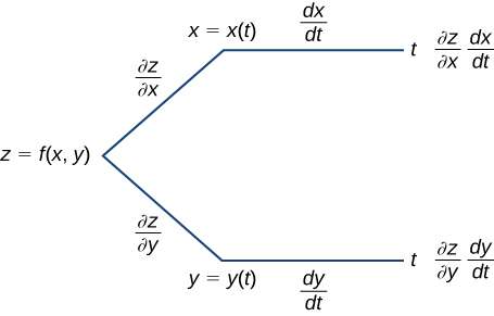
In this diagram, the leftmost corner corresponds to $z=f(x,y)$. Since $f$ has two independent variables, there are two lines coming from this corner. The upper branch corresponds to the variable $x$ and the lower branch corresponds to the variable $y$. Since each of these variables is then dependent on one variable $t$, one branch then comes from $x$ and one branch comes from $y$. Last, each of the branches on the far right has a label that represents the path traveled to reach that branch. The top branch is reached by following the $x$ branch, then the t branch; therefore, it is labeled $(∂z/∂x)×(dx/dt).$ The bottom branch is similar: first the $y$ branch, then the $t$ branch. This branch is labeled $(∂z/∂y)×(dy/dt)$. To get the formula for $dz/dt,$ add all the terms that appear on the rightmost side of the diagram. This gives us Equation.

In Chain Rule for Two Independent Variables, $z=f(x,y)$ is a function of $x$ and $y$, and both $x=g(u,v)$ and $y=h(u,v)$ are functions of the independent variables $u$ and $v$.

Theorem $\PageIndex{2}$: Chain Rule for Two Independent Variables

Suppose $x=g(u,v)$ and $y=h(u,v)$ are differentiable functions of $u$ and $v$, and $z=f(x,y)$ is a differentiable function of $x$ and $y$. Then, $z=f(g(u,v),h(u,v))$ is a differentiable function of $u$ and $v$, and

$$\dfrac{∂z}{∂u}=\dfrac{∂z}{∂x}\dfrac{∂x}{∂u}+\dfrac{∂z}{∂y}\dfrac{∂y}{∂u} \label{chain2a}$$

and

$$\dfrac{∂z}{∂v}=\dfrac{∂z}{∂x}\dfrac{∂x}{∂v}+\dfrac{∂z}{∂y}\dfrac{∂y}{∂v}. \label{chain2b}$$

We can draw a tree diagram for each of these formulas as well as follows.

Figure $\PageIndex{2}$: Tree diagram for $\dfrac{∂z}{∂u}=\dfrac{∂z}{∂x}⋅\dfrac{∂x}{∂u}+\dfrac{∂z}{∂y}⋅\dfrac{∂y}{∂u}$ and $\dfrac{∂z}{∂v}=\dfrac{∂z}{∂x}⋅\dfrac{∂x}{∂v}+\dfrac{∂z}{∂y}⋅\dfrac{∂y}{∂v}$.

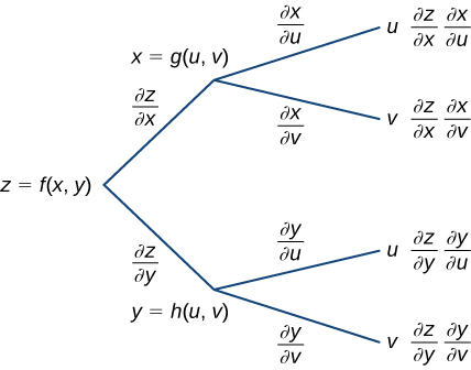
To derive the formula for $∂z/∂u$, start from the left side of the diagram, then follow only the branches that end with $u$ and add the terms that appear at the end of those branches. For the formula for $∂z/∂v$, follow only the branches that end with $v$ and add the terms that appear at the end of those branches.

There is an important difference between these two chain rule theorems. In Chain Rule for One Independent Variable, the left-hand side of the formula for the derivative is not a partial derivative, but in Chain Rule for Two Independent Variables it is. The reason is that, in Chain Rule for One Independent Variable, $z$ is ultimately a function of $t$ alone, whereas in Chain Rule for Two Independent Variables, $z$ is a function of both $u$ and $v$.

Example $\PageIndex{2}$: Using the Chain Rule for Two Variables

Calculate $∂z/∂u$ and $∂z/∂v$ using the following functions:

$$z=f(x,y)=3x^2−2xy+y^2,\; x=x(u,v)=3u+2v,\; y=y(u,v)=4u−v. \nonumber$$

Solution

To implement the chain rule for two variables, we need six partial derivatives—$∂z/∂x,\; ∂z/∂y,\; ∂x/∂u,\; ∂x/∂v,\; ∂y/∂u,$ and $∂y/∂v$:

$$\begin{align*} \dfrac{∂z}{∂x} &=6x−2y & & \dfrac{∂z}{∂y}=−2x+2y \\[4pt] \dfrac{∂x}{∂u} &=3 & & \dfrac{∂x}{∂v}=2 \\[4pt] \dfrac{∂y}{∂u} &=4 & & \dfrac{∂y}{∂v}=−1. \end{align*}$$

To find $∂z/∂u,$ we use Equation $\ref{chain2a}$:

$$\begin{align*} \dfrac{∂z}{∂u} &=\dfrac{∂z}{∂x}⋅\dfrac{∂x}{∂u}+\dfrac{∂z}{∂y}⋅\dfrac{∂y}{∂u} \\[4pt] &=3(6x−2y)+4(−2x+2y) \\[4pt] &=10x+2y. \end{align*}$$

Next, we substitute $x(u,v)=3u+2v$ and $y(u,v)=4u−v:$

$$\begin{align*} \dfrac{∂z}{∂u} &=10x+2y \\[4pt] &=10(3u+2v)+2(4u−v) \\[4pt] &=38u+18v. \end{align*}$$

To find $∂z/∂v,$ we use Equation $\ref{chain2b}$:

$$\begin{align*} \dfrac{∂z}{∂v} &=\dfrac{∂z}{∂x}\dfrac{∂x}{∂v}+\dfrac{∂z}{∂y}\dfrac{∂y}{∂v} \\[4pt] &=2(6x−2y)+(−1)(−2x+2y) \\[4pt] &=14x−6y. \end{align*}$$

Then we substitute $x(u,v)=3u+2v$ and $y(u,v)=4u−v:$

$$\begin{align*} \dfrac{∂z}{∂v} &=14x−6y \\[4pt] &=14(3u+2v)−6(4u−v) \\[4pt] &=18u+34v \end{align*}$$

Exercise $\PageIndex{2}$

Calculate $∂z/∂u$ and $∂z/∂v$ given the following functions:

$$z=f(x,y)=\dfrac{2x−y}{x+3y},\quad x(u,v)=e^{2u}\cos 3v,\quad y(u,v)=e^{2u}\sin 3v. \nonumber$$

Hint

Calculate $∂z/∂x,\; ∂z/∂y,\; ∂x/∂u,\; ∂x/∂v,\; ∂y/∂u,$ and $∂y/∂v$, then use Equation $\ref{chain2a}$ and Equation $\ref{chain2b}$.

Answer

$\dfrac{∂z}{∂u}=0,\quad \dfrac{∂z}{∂v}=\dfrac{−21}{(3\sin 3v+\cos 3v)^2}$

The Generalized Chain Rule

Now that we’ve see how to extend the original chain rule to functions of two variables, it is natural to ask: Can we extend the rule to more than two variables? The answer is yes, as the generalized chain rule states.

Theorem $\PageIndex{3}$: Generalized Chain Rule

Let $w=f(x_1,x_2,…,x_m)$ be a differentiable function of $m$ independent variables, and for each $i∈{1,…,m},$ let $x_i=x_i(t_1,t_2,…,t_n)$ be a differentiable function of $n$ independent variables. Then

$$\dfrac{∂w}{∂t_j}=\dfrac{∂w}{∂x_1}\dfrac{∂x_1}{∂t_j}+\dfrac{∂w}{∂x_2}\dfrac{∂x_2}{∂t_j}+⋯+\dfrac{∂w}{∂x_m}\dfrac{∂x_m}{∂t_j} \nonumber$$

for any $j∈{1,2,…,n}.$

In the next example we calculate the derivative of a function of three independent variables in which each of the three variables is dependent on two other variables.

Example $\PageIndex{3}$: Using the Generalized Chain Rule

Calculate $∂w/∂u$ and $∂w/∂v$ using the following functions:

$$\begin{align*} w &=f(x,y,z)=3x^2−2xy+4z^2 \\[4pt] x &=x(u,v)=e^u\sin v \\[4pt] y &=y(u,v)=e^u\cos v \\[4pt] z &=z(u,v)=e^u. \end{align*}$$

Solution

The formulas for $∂w/∂u$ and $∂w/∂v$ are

$$\begin{align*} \dfrac{∂w}{∂u} =\dfrac{∂w}{∂x}⋅\dfrac{∂x}{∂u}+\dfrac{∂w}{∂y}⋅\dfrac{∂y}{∂u}+\dfrac{∂w}{∂z}⋅\dfrac{∂z}{∂u} \\[4pt] \dfrac{∂w}{∂v} =\dfrac{∂w}{∂x}⋅\dfrac{∂x}{∂v}+\dfrac{∂w}{∂y}⋅\dfrac{∂y}{∂v}+\dfrac{∂w}{∂z}⋅\dfrac{∂z}{∂v}. \end{align*}$$

Therefore, there are nine different partial derivatives that need to be calculated and substituted. We need to calculate each of them:

$$\begin{align*} \dfrac{∂w}{∂x}&=6x−2y \dfrac{∂w}{∂y}=−2x \dfrac{∂w}{∂z}=8z \\[4pt] \dfrac{∂x}{∂u}&=e^u\sin v \dfrac{∂y}{∂u}=e^u\cos v \dfrac{∂z}{∂u}=e^u \\[4pt] \dfrac{∂x}{∂v}&=e^u\cos v \dfrac{∂y}{∂v}=−e^u\sin v \dfrac{∂z}{∂v}=0. \end{align*}$$

Now, we substitute each of them into the first formula to calculate $∂w/∂u$:

$$\begin{align*} \dfrac{∂w}{∂u} &=\dfrac{∂w}{∂x}⋅\dfrac{∂x}{∂u}+\dfrac{∂w}{∂y}⋅\dfrac{∂y}{∂u}+\dfrac{∂w}{∂z}⋅\dfrac{∂z}{∂u} \\[4pt] &=(6x−2y)e^u\sin v−2xe^u\cos v+8ze^u, \end{align*}$$

then substitute $x(u,v)=e^u \sin v, \, y(u,v)=e^u\cos v,$ and $z(u,v)=e^u$ into this equation:

$$\begin{align*} \dfrac{∂w}{∂u} &=(6x−2y)e^u\sin v−2xe^u\cos v+8ze^u \\[4pt] &=(6e^u\sin v−2eu\cos v)e^u\sin v−2(e^u\sin v)e^u\cos v+8e^{2u} \\[4pt] &=6e^{2u}\sin^2 v−4e^{2u}\sin v\cos v+8e^{2u} \\[4pt] &=2e^{2u}(3\sin^2 v−2\sin v\cos v+4). \end{align*}$$

Next, we calculate $∂w/∂v$:

$$\begin{align*} \dfrac{∂w}{∂v} &=\dfrac{∂w}{∂x}⋅\dfrac{∂x}{∂v}+\dfrac{∂w}{∂y}⋅\dfrac{∂y}{∂v}+\dfrac{∂w}{∂z}⋅\dfrac{∂z}{∂v} \\[4pt] &=(6x−2y)e^u\cos v−2x(−e^u\sin v)+8z(0), \end{align*}$$

then we substitute $x(u,v)=e^u\sin v,\, y(u,v)=e^u\cos v,$ and $z(u,v)=e^u$ into this equation:

$$\begin{align*} \dfrac{∂w}{∂v} &=(6x−2y)e^u\cos v−2x(−e^u\sin v) \\[4pt] &=(6e^u \sin v−2e^u\cos v)e^u\cos v+2(e^u\sin v)(e^u\sin v) \\[4pt] &=2e^{2u}\sin^2 v+6e^{2u}\sin v\cos v−2e^{2u}\cos^2 v \\[4pt] &=2e^{2u}(\sin^2 v+\sin v\cos v−\cos^2 v). \end{align*}$$

Exercise $\PageIndex{3}$

Calculate $∂w/∂u$ and $∂w/∂v$ given the following functions:

$$\begin{align*} w &=f(x,y,z)=\dfrac{x+2y−4z}{2x−y+3z} \\[4pt] x &=x(u,v)=e^{2u}\cos3v \\[4pt] y &=y(u,v)=e^{2u}\sin 3v \\[4pt] z &=z(u,v)=e^{2u}. \end{align*}$$

Hint

Calculate nine partial derivatives, then use the same formulas from Example $\PageIndex{3}$.

Answer

$\dfrac{∂w}{∂u}=0$

$\dfrac{∂w}{∂v}=\dfrac{15−33\sin 3v+6\cos 3v}{(3+2\cos 3v−\sin 3v)^2}$

Example $\PageIndex{4}$: Drawing a Tree Diagram

Create a tree diagram for the case when

$$w=f(x,y,z),\quad x=x(t,u,v),\quad y=y(t,u,v),\quad z=z(t,u,v) \nonumber$$

and write out the formulas for the three partial derivatives of $w$.

Solution

Starting from the left, the function $f$ has three independent variables: $x,\, y$, and $z$. Therefore, three branches must be emanating from the first node. Each of these three branches also has three branches, for each of the variables $t,\, u,$ and $v$.

Figure $\PageIndex{3}$: Tree diagram for a function of three variables, each of which is a function of three independent variables.

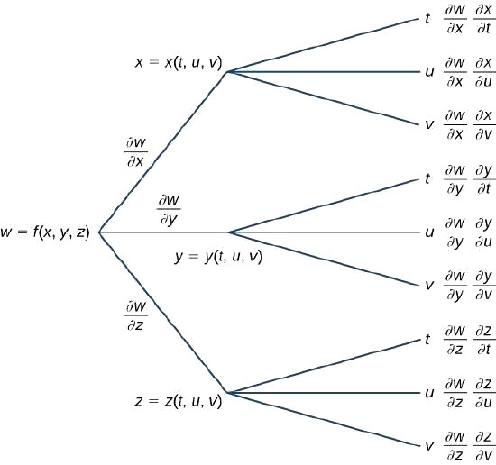
The three formulas are

$$\begin{align*} \dfrac{∂w}{∂t} &=\dfrac{∂w}{∂x}\dfrac{∂x}{∂t}+\dfrac{∂w}{∂y}\dfrac{∂y}{∂t}+\dfrac{∂w}{∂z}\dfrac{∂z}{∂t} \\[4pt] \dfrac{∂w}{∂u} &=\dfrac{∂w}{∂x}\dfrac{∂x}{∂u}+\dfrac{∂w}{∂y}\dfrac{∂y}{∂u}+\dfrac{∂w}{∂z}\dfrac{∂z}{∂u} \\[4pt] \dfrac{∂w}{∂v} &=\dfrac{∂w}{∂x}\dfrac{∂x}{∂v}+\dfrac{∂w}{∂y}\dfrac{∂y}{∂v}+\dfrac{∂w}{∂z}\dfrac{∂z}{∂v}. \end{align*}$$

Exercise $\PageIndex{4}$

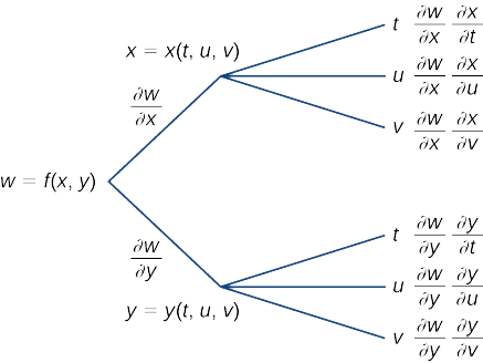
Create a tree diagram for the case when

$$w=f(x,y),\quad x=x(t,u,v),\quad y=y(t,u,v) \nonumber$$

and write out the formulas for the three partial derivatives of $w.$

Hint

Determine the number of branches that emanate from each node in the tree.

Answer

$$\begin{align*}\dfrac{∂w}{∂t} &=\dfrac{∂w}{∂x}\dfrac{∂x}{∂t}+\dfrac{∂w}{∂y}\dfrac{∂y}{∂t} \\[4pt] \dfrac{∂w}{∂u} &=\dfrac{∂w}{∂x}\dfrac{∂x}{∂u}+\dfrac{∂w}{∂y}\dfrac{∂y}{∂u} \\[4pt] \dfrac{∂w}{∂v} &=\dfrac{∂w}{∂x}\dfrac{∂x}{∂v}+\dfrac{∂w}{∂y}\dfrac{∂y}{∂v} \end{align*}$$

Implicit Differentiation

Recall from implicit differentiation provides a method for finding $dy/dx$ when $y$ is defined implicitly as a function of $x$. The method involves differentiating both sides of the equation defining the function with respect to $x$, then solving for $dy/dx.$ Partial derivatives provide an alternative to this method.

Consider the ellipse defined by the equation $x^2+3y^2+4y−4=0$ as follows.

Figure $\PageIndex{4}$: Graph of the ellipse defined by $x^2+3y^2+4y−4=0$.

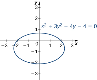
This equation implicitly defines $y$ as a function of $x$. As such, we can find the derivative $dy/dx$ using the method of implicit differentiation:

$$\begin{align*} \dfrac{d}{dx}(x^2+3y^2+4y−4) &=\dfrac{d}{dx}(0) \\[4pt] 2x+6y\dfrac{dy}{dx}+4\dfrac{dy}{dx} &=0 \\[4pt] (6y+4)\dfrac{dy}{dx} &=−2x\\[4pt] \dfrac{dy}{dx} &=−\dfrac{x}{3y+2}\end{align*}$$

We can also define a function $z=f(x,y)$ by using the left-hand side of the equation defining the ellipse. Then $f(x,y)=x^2+3y^2+4y−4.$ The ellipse $x^2+3y^2+4y−4=0$ can then be described by the equation $f(x,y)=0$. Using this function and the following theorem gives us an alternative approach to calculating $dy/dx.$

Theorem $\PageIndex{4}$: Implicit Differentiation of a Function of Two or More Variables

Suppose the function $z=f(x,y)$ defines $y$ implicitly as a function $y=g(x)$ of $x$ via the equation $f(x,y)=0.$ Then

$$\dfrac{dy}{dx}=−\dfrac{∂f/∂x}{∂f/∂y} \label{implicitdiff1}$$

provided $f_y(x,y)≠0.$

If the equation $f(x,y,z)=0$ defines $z$ implicitly as a differentiable function of $x$ and $y$, then

$$\dfrac{dz}{dx}=−\dfrac{∂f/∂x}{∂f/∂z} \qquad\text{and}\qquad \dfrac{dz}{dy}=−\dfrac{∂f/∂y}{∂f/∂z}\label{implicitdiff2}$$

as long as $f_z(x,y,z)≠0.$

Equation $\ref{implicitdiff1}$ is a direct consequence of Equation $\ref{chain2a}$. In particular, if we assume that $y$ is defined implicitly as a function of $x$ via the equation $f(x,y)=0$, we can apply the chain rule to find $dy/dx:$

$$\begin{align*} \dfrac{d}{dx}f(x,y) &=\dfrac{d}{dx}(0) \\[4pt] \dfrac{∂f}{∂x}⋅\dfrac{dx}{dx}+\dfrac{∂f}{∂y}⋅\dfrac{dy}{dx} &=0 \\[4pt]\dfrac{∂f}{∂x}+\dfrac{∂f}{∂y}⋅\dfrac{dy}{dx} &=0. \end{align*}$$

Solving this equation for $dy/dx$ gives Equation $\ref{implicitdiff1}$. Equation $\ref{implicitdiff1}$ can be derived in a similar fashion.

Let’s now return to the problem that we started before the previous theorem. Using Theorem $\PageIndex{4}$ and the function $f(x,y)=x^2+3y^2+4y−4,$ we obtain

$$\begin{align*} \dfrac{∂f}{∂x} &=2x\\[4pt] \dfrac{∂f}{∂y} &=6y+4. \end{align*}$$

Then Equation $\ref{implicitdiff1}$ gives

$$\dfrac{dy}{dx}=−\dfrac{∂f/∂x}{∂f/∂y}=−\dfrac{2x}{6y+4}=−\dfrac{x}{3y+2}, \nonumber$$

which is the same result obtained by the earlier use of implicit differentiation.

Example $\PageIndex{5}$: Implicit Differentiation by Partial Derivatives

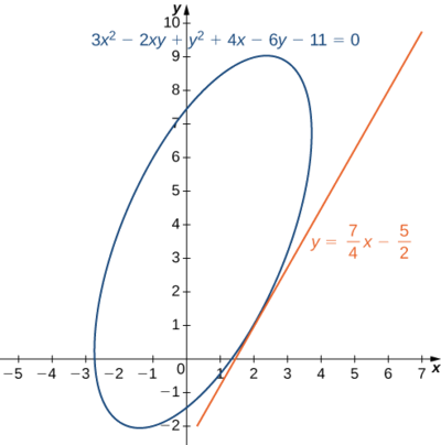
1. Calculate $dy/dx$ if $y$ is defined implicitly as a function of $x$ via the equation $3x^2−2xy+y^2+4x−6y−11=0$. What is the equation of the tangent line to the graph of this curve at point $(2,1)$?
2. Calculate $∂z/∂x$ and $∂z/∂y,$ given $x^2e^y−yze^x=0.$

Solution

a. Set $f(x,y)=3x^2−2xy+y^2+4x−6y−11=0,$ then calculate $f_x$ and $f_y: f_x(x,y)=6x−2y+4$ and $f_y(x,y)=−2x+2y−6.$

The derivative is given by

$$\dfrac{dy}{dx}=−\dfrac{∂f/∂x}{∂f/∂y}=\dfrac{6x−2y+4}{−2x+2y−6}=\dfrac{3x−y+2}{x−y+3}. \nonumber$$

The slope of the tangent line at point $(2,1)$ is given by

$$\dfrac{dy}{dx}\Bigg|_{(x,y)=(2,1)}=\dfrac{3(2)−1+2}{2−1+3}=\dfrac{7}{4} \nonumber$$

To find the equation of the tangent line, we use the point-slope form (Figure $\PageIndex{5}$):

$$\begin{align*} y−y_0 &=m(x−x_0)\\[4pt]y−1 &=\dfrac{7}{4}(x−2) \\[4pt] y &=\dfrac{7}{4}x−\dfrac{7}{2}+1\\[4pt] y &=\dfrac{7}{4}x−\dfrac{5}{2}.\end{align*}$$

Figure $\PageIndex{5}$: Graph of the rotated ellipse defined by $3x^2−2xy+y^2+4x−6y−11=0$.

b. We have $f(x,y,z)=x^2e^y−yze^x.$ Therefore,

$$\begin{align*} \dfrac{∂f}{∂x} &=2xe^y−yze^x \\[4pt] \dfrac{∂f}{∂y} &=x^2e^y−ze^x \\[4pt] \dfrac{∂f}{∂z} &=−ye^x\end{align*}$$

Using Equation $\ref{implicitdiff2}$,

$$\begin{align*} \dfrac{∂z}{∂x} &=−\dfrac{∂f/∂x}{∂f/∂y} & &\text{and} & \dfrac{∂z}{∂y} =−\dfrac{∂f/∂y}{∂f/∂z} \\[4pt] &=−\dfrac{2xe^y−yze^x}{−ye^x} & & &=−\dfrac{x^2e^y−ze^x}{−ye^x} \\[4pt] &=\dfrac{2xe^y−yze^x}{ye^x} & & & =\dfrac{x^2e^y−ze^x}{ye^x} \end{align*}$$

Exercise $\PageIndex{5}$

Find $dy/dx$ if $y$ is defined implicitly as a function of $x$ by the equation $x^2+xy−y^2+7x−3y−26=0$. What is the equation of the tangent line to the graph of this curve at point $(3,−2)$?

Hint

Calculate $∂f/dx$ and $∂f/dy$, then use Equation $\ref{implicitdiff1}$.

Solution

$$\dfrac { d y } { d x } = \left. \frac { 2 x + y + 7 } { 2 y - x + 3 } \right| _ { ( 3 , - 2 ) } = \dfrac { 2 ( 3 ) + ( - 2 ) + 7 } { 2 ( - 2 ) - ( 3 ) + 3 } = - \dfrac { 11 } { 4 } \nonumber$$

Equation of the tangent line: $y=−\dfrac{11}{4}x+\dfrac{25}{4}$

Key Concepts

• The chain rule for functions of more than one variable involves the partial derivatives with respect to all the independent variables.
• Tree diagrams are useful for deriving formulas for the chain rule for functions of more than one variable, where each independent variable also depends on other variables.

Key Equations

• Chain rule, one independent variable

$\dfrac{dz}{dt}=\dfrac{∂z}{∂x}⋅\dfrac{dx}{dt}+\dfrac{∂z}{∂y}⋅\dfrac{dy}{dt}$

• Chain rule, two independent variables

$\dfrac{dz}{du}=\dfrac{∂z}{∂x}⋅\dfrac{∂x}{∂u}+\dfrac{∂z}{∂y}⋅\dfrac{∂y}{∂u}\dfrac{dz}{dv}=\dfrac{∂z}{∂x}⋅\dfrac{∂x}{∂v}+\dfrac{∂z}{∂y}⋅\dfrac{∂y}{∂v}$

• Generalized chain rule

$\dfrac{∂w}{∂t_j}=\dfrac{∂w}{∂x_1}\dfrac{∂x_1}{∂t_j}+\dfrac{∂w}{∂x_2}\dfrac{∂x_1}{∂t_j}+⋯+\dfrac{∂w}{∂x_m}\dfrac{∂x_m}{∂t_j}$

Glossary

generalized chain rule

the chain rule extended to functions of more than one independent variable, in which each independent variable may depend on one or more other variables

intermediate variable

given a composition of functions (e.g., $f(x(t),y(t)))$, the intermediate variables are the variables that are independent in the outer function but dependent on other variables as well; in the function $f(x(t),y(t)),$ the variables $x$ and $y$ are examples of intermediate variables

tree diagram

illustrates and derives formulas for the generalized chain rule, in which each independent variable is accounted for