16.2: Line Integrals

In single-variable calculus you learned how to integrate a real-valued function \(f (x)\) over an interval \([a,b]\) in \(\mathbb{R}^1\). This integral (usually called a Riemann integral) can be thought of as an integral over a path in \(\mathbb{R}^1\), since an interval (or collection of intervals) is really the only kind of “path” in \(\mathbb{R}^1\). You may also recall that if \(f (x)\) represented the force applied along the \(x\)-axis to an object at position \(x\) in \([a,b]\), then the work \(W\) done in moving that object from position \(x = a \text{ to }x = b\) was defined as the integral:

\[W=\int_a^b f (x)dx\]

In this section, we will see how to define the integral of a function (either real-valued or vector-valued) of two variables over a general path (i.e. a curve) in \(\mathbb{R}^2\). This definition will be motivated by the physical notion of work. We will begin with real-valued functions of two variables.

In physics, the intuitive idea of work is that

\[\text{Work = Force × Distance}\]

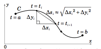
Suppose that we want to find the total amount \(W\) of work done in moving an object along a curve \(C\) in \(\mathbb{R}^2\) with a smooth parametrization \(x = x(t), y = y(t), a ≤ t ≤ b\), with a force \(f (x, y)\) which varies with the position \((x, y)\) of the object and is applied in the direction of motion along \(C\) (see Figure \(\PageIndex{1}\) below).

Figure \(\PageIndex{1}\) Curve \(C : x = x(t),\, y = y(t) \text{ for }t \text{ in }[a,b]\)

We will assume for now that the function \(f (x, y)\) is continuous and real-valued, so we only consider the magnitude of the force. Partition the interval \([a,b]\) as follows:

\[a = t_0 < t_1 < t_2 < ··· < t_{n−1} < t_n = b ,\text{ for some integer }n ≥ 2\]

As we can see from Figure \(\PageIndex{1}\), over a typical subinterval \([t_i ,t_{i+1}]\) the distance \(∆s_i\) traveled along the curve is approximately \(\sqrt{∆x_i^2 +∆y_i^2}\), by the Pythagorean Theorem. Thus, if the subinterval is small enough then the work done in moving the object along that piece of the curve is approximately

\[\text{Force × Distance} \approx f (x_{i∗}, y_{i∗}) \sqrt{ ∆x_i^2 +∆y_i^2}\label{Eq4.1}\]

where \((x_{i∗}, y_{i∗}) = (x(t_{i∗}), y(t_{i∗}))\) for some \(t_{i∗} \text{ in }[t_i ,t_{i+1}]\), and so

\[W \approx \sum_{i=0}^{n-1} f (x_{i∗}, y_{i∗}) \sqrt{ ∆x_i^2 +∆y_i^2}\label{Eq4.2}\]

is approximately the total amount of work done over the entire curve. But since

\[\sqrt{ ∆x_i^2 +∆y_i^2} = \sqrt{\left ( \dfrac{∆x_i}{∆t_i} \right )^2 +\left ( \dfrac{∆y_i}{∆t_i}\right )^2}∆t_i\]

where \(∆t_i = t_{i+1} − t_i\), then

\[W \approx \sum_{i=0}^{n-1}f (x_{i∗}, y_{i∗})\sqrt{\left ( \dfrac{∆x_i}{∆t_i} \right )^2 + \left ( \dfrac{∆y_i}{∆t_i} \right )^2}∆t_i \label{Eq4.3}\]

Taking the limit of that sum as the length of the largest subinterval goes to 0, the sum over all subintervals becomes the integral from \(t = a \text{ to }t = b\), \(∆x_i ∆t_i \text{ and }∆y_i ∆t_i\) become \(x ′ (t) \text{ and }y ′ (t)\), respectively, and \(f (x_{i∗}, y_{i∗})\) becomes \(f (x(t), y(t))\), so that

\[W=\int_a^b f (x(t), y(t)) \sqrt{x ′ (t)^2 + y ′ (t)^2}\,dt \label{Eq4.4}\]

The integral on the right side of the above equation gives us our idea of how to define, for any real-valued function \(f (x, y)\), the integral of \(f (x, y)\) along the curve \(C\), called a line integral:

Definition \(\PageIndex{1}\): Line Integral of a scalar Field

For a real-valued function \(f (x, y)\) and a curve \(C\) in \(\mathbb{R}^2\), parametrized by \(x = x(t), y = y(t), a ≤ t ≤ b\), the line integral of \(f (x, y)\) along \(C\) with respect to arc length \(s\) is

\[\int_C f (x, y)\,ds = \int_a^b f (x(t), y(t))\sqrt{x ′ (t)^2 + y ′ (t)^2}\,dt \label{Eq4.5}\]

The symbol \(ds\) is the differential of the arc length function

\[s = s(t) = \int_a^t \sqrt{x ′ (u)^2 + y ′ (u)^2}\,du \label{Eq4.6}\]

which you may recognize from Section 1.9 as the length of the curve \(C\) over the interval \([a,t]\), for all \(t\) in \([a,b]\). That is,

\[ds = s ′ (t)\,dt = \sqrt{x ′ (t)^2 + y ′ (t)^2}\,dt, \label{Eq4.7}\]

by the Fundamental Theorem of Calculus.

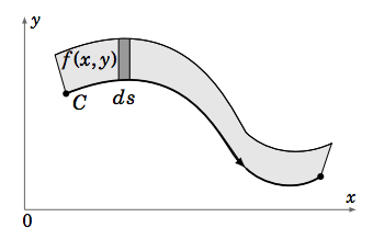
For a general real-valued function \(f (x, y)\), what does the line integral \(\int_C f (x, y)\,ds\) represent? The preceding discussion of \(ds\) gives us a clue. You can think of differentials as infinitesimal lengths. So if you think of \(f (x, y)\) as the height of a picket fence along \(C\), then \(f (x, y)\,ds\) can be thought of as approximately the area of a section of that fence over some infinitesimally small section of the curve, and thus the line integral \(\int_C f (x, y)\,ds\) is the total area of that picket fence (see Figure \(\PageIndex{2}\)).

Figure \(\PageIndex{2}\): Area of shaded rectangle = height × width ≈ \(f (x, y)\,ds\)

Example \(\PageIndex{1}\)

Use a line integral to show that the lateral surface area \(A\) of a right circular cylinder of radius \(r\) and height \(h\) is \(2\pi rh\).

Solution

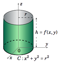
We will use the right circular cylinder with base circle \(C\) given by \(x^2 + y^2 = r^2\) and with height \(h\) in the positive \(z\) direction (see Figure \(\PageIndex{3}\)). Parametrize \(C\) as follows:

\[x = x(t) = r \cos t , y = y(t) = r \sin t , 0 ≤ t ≤ 2π\]

Figure \(\PageIndex{3}\)

\[\nonumber \begin{align} A&=\int_C f (x, y)\,ds = \int_a^b f (x(t), y(t))\sqrt{x ′ (t)^2 + y ′ (t)^2}\,dt \\[4pt] \nonumber &=\int_0^{2\pi} h \sqrt{(−r \sin t)^2 +(r \cos t)^2}\,dt \\[4pt] \nonumber &=h\int_0^{2\pi} r \sqrt{\sin^2 t+\cos^2 t}\,dt \\[4pt] \nonumber &=rh\int_0^{2\pi} 1\,dt = 2\pi rh \\[4pt] \end{align}\]

Note in Example \(\PageIndex{1}\) that if we had traversed the circle \(C\) twice, i.e. let t vary from \(0 \text{ to }4\pi\) then we would have gotten an area of \(4\pi rh\), i.e. twice the desired area, even though the curve itself is still the same (namely, a circle of radius \(r\)). Also, notice that we traversed the circle in the counter-clockwise direction. If we had gone in the clockwise direction, using the parametrization

\[x = x(t) = r \cos (2π− t) , y = y(t) = r \sin (2π− t) , 0 ≤ t ≤ 2π ,\label{Eq4.8}\]

then it is easy to verify (Exercise 12) that the value of the line integral is unchanged.

In general, it can be shown (Exercise 15) that reversing the direction in which a curve \(C\) is traversed leaves \(\int_C f (x, y)\,ds\) unchanged, for any \(f (x, y)\). If a curve \(C\) has a parametrization \(x = x(t), y = y(t), a ≤ t ≤ b,\) then denote by \(−C\) the same curve as \(C\) but traversed in the opposite direction. Then \(−C\) is parametrized by

\[x = x(a+ b − t) , y = y(a+ b − t) , a ≤ t ≤ b ,\label{Eq4.9}\]

and we have

\[\int_C f (x, y)\,ds =\int_{-C}f (x, y)\,ds .\label{Eq4.10}\]

Notice that our definition of the line integral was with respect to the arc length parameter \(s\). We can also define

\[\int_C f (x, y)\,dx=\int_a^b f (x(t), y(t)) x ′ (t)\,dt\label{Eq4.11}\]

as the line integral of \(f (x, y)\) along \(C\) with respect to \(x\), and

\[\int_C f (x, y)\,d y=\int_a^b f (x(t), y(t)) y ′ (t)\,dt \label{Eq4.12}\]

as the line integral of \(f (x, y)\) along \(C\) with respect to \(y\).

In the derivation of the formula for a line integral, we used the idea of work as force multiplied by distance. However, we know that force is actually a vector. So it would be helpful to develop a vector form for a line integral. For this, suppose that we have a function \(f(x, y)\) defined on \(\mathbb{R}^2\) by

\[\nonumber \textbf{f}(x, y) = P(x, y)\textbf{i} + Q(x, y)\textbf{j}\]

for some continuous real-valued functions \(P(x, y)\) and \(Q(x, y) \text{ on }\mathbb{R}^2\). Such a function \(f\) is called a vector field on \(\mathbb{R}^2\). It is defined at points in \(\mathbb{R}^2\), and its values are vectors in \(\mathbb{R}^2\). For a curve \(C\) with a smooth parametrization \(x = x(t), y = y(t), a ≤ t ≤ b\), let

\[\nonumber \textbf{r}(t) = x(t)\textbf{i} + y(t)\textbf{j}\]

be the position vector for a point \((x(t), y(t))\) on \(C\). Then \(\textbf{r}'(t) = x'(t)\textbf{i} + y'(t)\textbf{j}\) and so

\[\nonumber \begin{align} \int_C P(x, y)\,dx+ \int_C Q(x, y)\,d y &=\int_a^b P(x(t), y(t)) x ′ (t)\,dt+\int_a^b Q(x(t), y(t)) y ′ (t)\,dt \\[4pt] \nonumber &=\int_a^b (P(x(t), y(t)) x ′ (t)+Q(x(t), y(t)) y ′ (t))\,dt \\[4pt] \nonumber &=\int_a^b \textbf{f}(x(t), y(t))\cdot \textbf{r} ′ (t)dt \\[4pt] \end{align}\]

by definition of \(f(x, y)\). Notice that the function \(f(x(t), y(t))\cdot r ′ (t)\) is a real-valued function on \([a,b]\), so the last integral on the right looks somewhat similar to our earlier definition of a line integral. This leads us to the following definition:

Definition \(\PageIndex{2}\): Line Integral of a vector Field

For a vector field \(\textbf{f}(x, y) = P(x, y)\textbf{i} +Q(x, y)\textbf{j}\) and a curve \(C\) with a smooth parametrization \(x = x(t), y = y(t), a ≤ t ≤ b\), the line integral of f along \(C\) is

\[\begin{align} \int_C \textbf{f}\cdot d\textbf{r} &= \int_C P(x, y)\,dx+\int_C Q(x, y)\,d y \label{Eq4.13} \\[4pt] &=\int_a^b \textbf{f}(x(t), y(t))\cdot \textbf{r} ′ (t)\,dt \label{Eq4.14} \\[4pt] \end{align}\]

where \(\textbf{r}(t) = x(t)\textbf{i}+ y(t)\textbf{j}\) is the position vector for points on \(C\).

We use the notation \(d\textbf{r} = \textbf{r} ′ (t)\,dt = dx\textbf{i}+ d y\textbf{j}\) to denote the differential of the vector-valued function r. The line integral in Definition \(\PageIndex{2}\) is often called a line integral of a vector field to distinguish it from the line integral in Definition \(\PageIndex{1}\) which is called a line integral of a scalar field. For convenience we will often write

\[\nonumber \int_C P(x, y)\,dx +\int_C Q(x, y)\,d y =\int_C P(x, y)\,dx+Q(x, y)\,d y ,\]

where it is understood that the line integral along \(C\) is being applied to both \(P \text{ and }Q\). The quantity \(P(x, y)\,dx +Q(x, y)\,d y\) is known as a differential form. For a real-valued function \(F(x, y)\), the differential of \(F\) is

\[dF = \dfrac{∂F}{∂x}\,dx+ \dfrac{∂F}{∂y}\, d y.\]

A differential form \(P(x, y)\,dx+Q(x, y)\,d y\) is called exact if it equals \(dF\) for some function \(F(x, y)\).

Recall that if the points on a curve \(C\) have position vector \(\textbf{r}(t) = x(t)\textbf{i}+ y(t)\textbf{j}\), then \(\textbf{r} ′ (t)\) is a tangent vector to \(C\) at the point \((x(t), y(t))\) in the direction of increasing \(t\) (which we call the direction of \(C\)). Since \(C\) is a smooth curve, then \(\textbf{r} ′ (t) \neq \textbf{0} \text{ on }[a,b]\) and hence

\[\nonumber \textbf{T}(t) = \dfrac{\textbf{r}'(t)}{\left \lVert \textbf{r}'(t) \right \rVert} \]

is the unit tangent vector to \(C\) at \((x(t), y(t))\). Putting Definitions \(\PageIndex{1}\) and \(\PageIndex{2}\) together we get the following theorem:

Theorem \(\PageIndex{1}\)

For a vector field \(\textbf{f}(x, y) = P(x, y)\textbf{i} + Q(x, y)\textbf{j}\) and a curve \(C\) with a smooth parametrization \(x = x(t), y = y(t), a ≤ t ≤ b\) and position vector \(\textbf{r}(t) = x(t)\textbf{i}+ y(t)\textbf{j}\),

\[\int_C \textbf{f}\cdot d\textbf{r} = \int_C \textbf{f}\cdot \textbf{T}\,ds,\label{Eq4.15}\]

where \(\textbf{T}(t) = \dfrac{\textbf{r} ′ (t)}{ \left \lVert \textbf{r} ′ (t)\right \rVert }\) is the unit tangent vector to \(C\) at \((x(t), y(t))\).

If the vector field \( \textbf{f}(x, y)\) represents the force moving an object along a curve \(C\), then the work \(W\) done by this force is

\[W = \int_C \textbf{f}\cdot \textbf{T} \, ds = \int_C \textbf{f}\cdot d\textbf{r} \label{Eq4.16}\]