The Method of Least Squares Regression (as an Application of Optimization)

Our world is full of data, and to interpret and extrapolate based on this data, we often try to find a function to model this data in a particular situation.  You've likely heard about a line of best fit, also known as a least squares regression line.  This linear model, in the form $f(x) = ax + b$, assumes the value of the output changes at a roughly constant rate with respect to the input, i.e., that these values are related linearly.  And for many situations this linear model gives us a powerful way to make predictions about the value of the function's output for inputs other than those in the data we collected.  For other situations, like most population models, a linear model is not sufficient, and we need to find a quadratic, cubic, exponential, logistic, or trigonometric model (or possibly something else).

Consider the data points given in the table below.  Figures $\PageIndex{11}$ -  $\PageIndex{14}$ show various best fit regression models for this data.

$\qquad \begin{array}{c  |  c}  x & y \\ \hline 2 & 1 \\ 4 & 2 \\ 6 & 4 \\ 8 & 7  \end{array}$

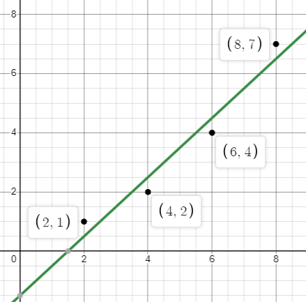
Figure $\PageIndex{11}$: Linear model

$y = x - 1.5$

Figure $\PageIndex{12}$: Quadratic model

$y = 0.125x^2 - 0.25x + 1$

Figure $\PageIndex{13}$: Exponential model

$y = 0.6061 \cdot (1.359)^x$

Figure $\PageIndex{14}$: Logistic model

$y = \dfrac{18.31}{1 + 39.67 e^{-0.4002 x}}$

Definition: Sum of the Squared Errors Function

One way to measure how well a particular model $y = f(x)$ fits a given set of data points $\big\{(x_1, y_1), (x_2, y_2), (x_3, y_3), ..., (x_n, y_n)\big\}$ is to consider the squares of the differences between the values given by the model and the actual $y$-values of the data points.

Figure $\PageIndex{15}$: Differences between model $y = f(x)$ and $y$-coordinates of data points, where $d_i = f(x_i) - y_i$.

The differences (or errors), $d_i = f(x_i) - y_i$, are squared and added up so that all errors are considered in the measure of how well the model "fits" the data.  This sum of the squared errors is given by

$$S = \sum_{i=1}^n \big( f(x_i) - y_i \big)^2 \nonumber$$

Squaring the errors in this sum also tends to magnify the weight of larger errors and minimize the weight of small errors in the measurement of how well the model fits the data.

Note that $S$ is a function of the constant parameters in the particular model $y = f(x)$.  For example, if we desire a linear model, then $f(x) = a x + b$, and

$$\begin{align*} S(a, b) &= \sum_{i=1}^n \big( f(x_i) - y_i \big)^2  \\ &= \sum_{i=1}^n \big( a x_i + b - y_i \big)^2 \end{align*}$$

To obtain the best fit version of the model, we will seek the values of the constant parameters in the model ($a$ and $b$ in the linear model) that give us the minimum value of this sum of the squared errors function $S$ for the given set of data points.

When calculating a line of best fit in previous classes, you were likely either given the formulas for the coefficients or shown how to use features on your calculator or other device to find them.

Using our understanding of the optimization of functions of multiple variables in this class, we are now able to derive the formulas for these coefficients directly.  In fact, we can use the same methods to determine the constant parameters needed to form a best fit model of any kind (quadratic, cubic, exponential, logistic, sine, cosine, etc), although these can be a bit more difficult to work out than the linear case.

Theorem $\PageIndex{2}$: Least Squares Regression Line

The least squares regression line (or line of best fit) for the data points $\big\{(x_1, y_1), (x_2, y_2), (x_3, y_3), ..., (x_n, y_n)\big\}$ is given by the formula

$$f(x) = ax + b \nonumber$$

where

$$a = \frac{\displaystyle {n \sum_{i=1}^n x_i y_i - \sum_{i=1}^n x_i \sum_{i=1}^n y_i}}{\displaystyle{n\sum_{i=1}^n {x_i}^2 - \left( \sum_{i=1}^n x_i \right)^2}} \qquad \text{and} \qquad b = \tfrac{1}{n}\left(\sum_{i=1}^n y_i - a\sum_{i=1}^n x_i \right). \nonumber$$

Proof (part 1): To obtain a line that best fits the data points we need to minimize the sum of the squared errors for this model.  This is a function of the two variables $a$ and $b$ as shown below.  Note that the $x_i$ and $y_i$ are numbers in this function and are not the variables.

$$S(a, b) = \sum_{i=1}^n \big( a x_i + b - y_i \big)^2 \nonumber$$

To minimize this function of the two variables $a$ and $b$, we need to determine the critical point(s) of this function.  Let's start by stating the partial derivatives of $S$ with respect to $a$ and $b$ and simplifying them so that the sums only include the numerical coordinates from the data points.

$$\begin{align*}  S_a(a, b) &= \sum_{i=1}^n 2x_i\big( a x_i + b - y_i \big) \\ &=  \sum_{i=1}^n \big( 2a {x_i}^2 + 2b x_i - 2x_i y_i \big) \\ &=  \sum_{i=1}^n 2a {x_i}^2   +  \sum_{i=1}^n 2b x_i -  \sum_{i=1}^n 2x_i y_i  \\ &= 2a \sum_{i=1}^n {x_i}^2   +  2b \sum_{i=1}^n x_i -  2 \sum_{i=1}^n x_i y_i    \end{align*}$$

$$\begin{align*}  S_b(a, b) &= \sum_{i=1}^n 2 \big( a x_i + b - y_i \big) \\ &=  \sum_{i=1}^n \big( 2a x_i + 2b - 2 y_i \big) \\ &=  \sum_{i=1}^n 2a x_i   +  \sum_{i=1}^n 2b -  \sum_{i=1}^n 2 y_i  \\ &= 2a \sum_{i=1}^n x_i   +  2b \sum_{i=1}^n 1 -  2 \sum_{i=1}^n y_i \\ &= 2a \sum_{i=1}^n x_i   +  2b n -  2 \sum_{i=1}^n y_i   \end{align*}$$

Next we set these partial derivatives equal to $0$ and solve the resulting system of equations.

Set $\displaystyle 2a \sum_{i=1}^n {x_i}^2   +  2b \sum_{i=1}^n x_i -  2 \sum_{i=1}^n x_i y_i  = 0$,

and $\displaystyle 2a \sum_{i=1}^n x_i   +  2b n -  2 \sum_{i=1}^n y_i = 0$.

Since the linear case is simple enough to make this process straightforward, we can use substitution to actually solve this system for $a$ and $b$.  Solving the second equation for $b$ gives us

$\qquad \displaystyle  2bn = 2 \sum_{i=1}^n y_i - 2a \sum_{i=1}^n x_i$

$\qquad \displaystyle  \boxed{b = \tfrac{1}{n}\left(\sum_{i=1}^n y_i - a\sum_{i=1}^n x_i \right).}$

We now substitute this expression into the first equation for $b$.

$\qquad \displaystyle 2a \sum_{i=1}^n {x_i}^2   +  2\left[\tfrac{1}{n}\left(\sum_{i=1}^n y_i - a\sum_{i=1}^n x_i \right)\right] \sum_{i=1}^n x_i -  2 \sum_{i=1}^n x_i y_i  = 0$

Multiplying this equation through by $n$ and dividing out the $2$ yields

$\qquad \displaystyle an \sum_{i=1}^n {x_i}^2   +  \left[\sum_{i=1}^n y_i - a\sum_{i=1}^n x_i \right] \sum_{i=1}^n x_i -  n \sum_{i=1}^n x_i y_i  = 0.$

Simplifying,

$\qquad \displaystyle an \sum_{i=1}^n {x_i}^2   +  \sum_{i=1}^n x_i \sum_{i=1}^n y_i - a\sum_{i=1}^n x_i \sum_{i=1}^n x_i -  n \sum_{i=1}^n x_i y_i  = 0.$

Next we isolate the terms containing $a$ on the left side of the equation, moving the other two terms to the right side of the equation.

$\qquad \displaystyle an \sum_{i=1}^n {x_i}^2   - a\left(\sum_{i=1}^n x_i\right)^2 =  n \sum_{i=1}^n x_i y_i  - \sum_{i=1}^n x_i \sum_{i=1}^n y_i.$

Factoring out the $a$,

$\qquad \displaystyle a\left( n \sum_{i=1}^n {x_i}^2   - \left(\sum_{i=1}^n x_i\right)^2\right) =  n \sum_{i=1}^n x_i y_i  - \sum_{i=1}^n x_i \sum_{i=1}^n y_i.$

Finally, we solve for $a$ to obtain

$\qquad \displaystyle \boxed{a = \frac{\displaystyle {n \sum_{i=1}^n x_i y_i - \sum_{i=1}^n x_i \sum_{i=1}^n y_i}}{\displaystyle{n\sum_{i=1}^n {x_i}^2 - \left( \sum_{i=1}^n x_i \right)^2}}.} \qquad$

$\qquad \qquad \qquad \qquad \qquad \qquad \qquad \qquad \blacksquare \qquad\text{QED}$        

 

Thus we have found formulas for the coordinates of the single critical point of the sum of squared errors function for the linear model, i.e.,

$\qquad \displaystyle S(a, b) = \sum_{i=1}^n \big( a x_i + b - y_i \big)^2$.

Proof (part 2): To prove that this linear model gives us a minimum of $S$, we will need the Second Partials Test.

The second partials of $S$ are

$$\begin{align*} S_{aa}(a,b) &= \sum_{i=1}^n 2{x_i}^2 \\ S_{bb}(a,b) &= \sum_{i=1}^n 2 = 2n \\ S_{ab}(a,b) &= \sum_{i=1}^n 2 x_i. \end{align*}$$

Then the discriminant evaluated at the critical point $(a, b)$ is

$$\begin{align*}  D(a, b) &= S_{aa}(a,b)  S_{bb}(a,b) - \big[ S_{ab}(a,b) \big]^2  \\ &= 2n \sum_{i=1}^n 2{x_i}^2  - \left( 2 \sum_{i=1}^n x_i \right)^2 \\ &= 4n \sum_{i=1}^n {x_i}^2 - 4 \left( \sum_{i=1}^n x_i \right)^2 \\ &= 4\left[  n \sum_{i=1}^n {x_i}^2 -  \left( \sum_{i=1}^n x_i \right)^2 \right]. \end{align*}$$

Now to prove that this discriminant is positive (and thus guarantees a local max or min) requires us to use the Cauchy-Schwarz Inequality.  This part of the proof is non-trivial, but not too hard, if we don't worry about proving the Cauchy-Schwarz Inequality itself here.

The Cauchy-Schwarz Inequality guarantees

$$\left(\sum_{i=1}^n a_i b_i\right)^2   \leq  \left(\sum_{i=1}^n {a_i}^2 \right) \left(\sum_{i=1}^n {b_i}^2 \right)\nonumber$$

for any real-valued sequences $a_i$ and $b_i$, with equality only if these two sequences are dependent (e.g., if the terms were the same or some multiple of each other).

Here we choose $a_i = 1$ and $b_i = x_i$.  Since these sequences are linearly independent, we will not have equality and substituting into the Cauchy-Schwarz Inequality gives us

$$\left(\sum_{i=1}^n 1 \cdot x_i \right)^2   <  \left(\sum_{i=1}^n {1}^2 \right) \left(\sum_{i=1}^n {x_i}^2 \right). \nonumber$$

Since $\displaystyle \sum_{i=1}^n 1 = n$, we have

$$\left(\sum_{i=1}^n x_i \right)^2   <  n \sum_{i=1}^n {x_i}^2.  \nonumber$$

This result proves

 

$$D(a,b) = 4\left[  n \sum_{i=1}^n {x_i}^2 -  \left( \sum_{i=1}^n x_i \right)^2 \right] > 0. \nonumber$$

Now, since it is clear that $\displaystyle S_{aa}(a,b) = \sum_{i=1}^n 2{x_i}^2 > 0$, we know that $S$ is concave up at the point $(a, b)$ and thus has a relative minimum there.  This concludes the proof that the parameters $a$ and $b$, as shown in Theorem $\PageIndex{2}$, give us the least squares linear regression model or line of best fit,

$$f(x) = ax + b.   \qquad \qquad \qquad \blacksquare \qquad\text{QED}  \nonumber$$

 

Note

The linear case $f(x)=ax+b$ is special in that it is simple enough to allow us to actually solve for the constant parameters $a$ and $b$ directly as formulas (as shown above in Theorem $\PageIndex{2}$.  For other best fit models we typically just obtain the system of equations needed to solve for the corresponding constant parameters that give us the critical point and minimum value of $S$.

To leave the quadratic regression case for you to try as an exercise, let's consider a cubic best fit model here.

Example $\PageIndex{6}$: Finding the System of Equations for the Best-fit Cubic Model

Determine the system of equations needed to determine the cubic best fit regression model of the form, $f(x) = ax^3 + bx^2 + cx + d$, for a given set of data points, $\big\{(x_1, y_1), (x_2, y_2), (x_3, y_3), ..., (x_n, y_n)\big\}$.

Solution

Here consider the sum of least squares function

$$S(a, b, c, d) = \sum_{i=1}^n \big( a {x_i}^3 + b {x_i}^2 + c x_i + d - y_i \big)^2. \nonumber$$

To find the minimum value of this function (and the corresponding values of the parameters $a, b, c,$ and $d$ needed for the best fit cubic regression model), we need to find the critical point of this function.  (Yes, even for a function of four variables!)  To begin this process, we find the first partial derivatives of this function with respect to each of the parameters $a, b, c,$ and $d$.

$$\begin{align*}  S_a(a, b, c, d) &= 2 \sum_{i=1}^n {x_i}^3 \big( a {x_i}^3 + b {x_i}^2 + c x_i + d - y_i \big) \\ S_b(a, b, c, d) &= 2 \sum_{i=1}^n {x_i}^2 \big( a {x_i}^3 + b {x_i}^2 + c x_i + d - y_i \big) \\ S_c(a, b, c, d) &= 2 \sum_{i=1}^n x_i \big( a {x_i}^3 + b {x_i}^2 + c x_i + d - y_i \big) \\ S_d(a, b, c, d) &= 2 \sum_{i=1}^n \big( a {x_i}^3 + b {x_i}^2 + c x_i + d - y_i \big)    \end{align*}$$

Now we set these partials equal to $0$, divide out the 2 from each, and split the terms into separate sums.  We also factor out the $a, b, c,$ and $d$ which don't change as the index changes.

$$\begin{align*}  a \sum_{i=1}^n {x_i}^6 + b \sum_{i=1}^n {x_i}^5 + c \sum_{i=1}^n {x_i}^4 + d\sum_{i=1}^n {x_i}^3 - \sum_{i=1}^n {x_i}^3 y_i = 0  \\ a \sum_{i=1}^n {x_i}^5 + b \sum_{i=1}^n {x_i}^4 + c \sum_{i=1}^n {x_i}^3 + d\sum_{i=1}^n {x_i}^2 - \sum_{i=1}^n {x_i}^2 y_i = 0  \\ a \sum_{i=1}^n {x_i}^4 + b \sum_{i=1}^n {x_i}^3 + c \sum_{i=1}^n {x_i}^2 + d\sum_{i=1}^n x_i - \sum_{i=1}^n x_i y_i = 0  \\ a \sum_{i=1}^n {x_i}^3 + b \sum_{i=1}^n {x_i}^2 + c \sum_{i=1}^n x_i + d\sum_{i=1}^n 1 - \sum_{i=1}^n y_i = 0  \\    \end{align*}$$

This system of equations can be rewritten by moving the negative terms to the right side of the equation.  We'll also emphasize the coefficients and variables and replace $\displaystyle \sum_{i=1}^n 1$ with $n$.

$$\begin{align*}  \left( \sum_{i=1}^n {x_i}^6 \right)a + \left( \sum_{i=1}^n {x_i}^5 \right) b + \left( \sum_{i=1}^n {x_i}^4 \right) c +\left(\sum_{i=1}^n {x_i}^3 \right) d = \sum_{i=1}^n {x_i}^3 y_i   \\  \left(\sum_{i=1}^n {x_i}^5 \right) a + \left( \sum_{i=1}^n {x_i}^4 \right) b + \left( \sum_{i=1}^n {x_i}^3 \right) c + \left(\sum_{i=1}^n {x_i}^2 \right) d = \sum_{i=1}^n {x_i}^2 y_i  \\  \left(\sum_{i=1}^n {x_i}^4 \right) a +\left( \sum_{i=1}^n {x_i}^3 \right) b + \left( \sum_{i=1}^n {x_i}^2 \right) c + \left( \sum_{i=1}^n x_i \right) d = \sum_{i=1}^n x_i y_i   \\  \left( \sum_{i=1}^n {x_i}^3 \right) a + \left( \sum_{i=1}^n {x_i}^2 \right) b +\left( \sum_{i=1}^n x_i \right) c + nd = \sum_{i=1}^n y_i   \\    \end{align*}$$

This is a system of four linear equations with the four variables $a, b, c,$ and $d$.  To solve for the values of these parameters that would give us the best fit cubic regression model, we would need to solve this system using the given data points.  We would first evaluate each of the sums using the $x$- and $y$-coordinates of the data points and place these numerical coefficients into the equations.  We would then only need to solve the resulting system of linear equations.

Let's now use this process to find the best fit cubic regression model for a set of data points.

Example $\PageIndex{7}$: Finding a Best-fit Cubic Model

a. Find the best fit cubic regression model of the form, $f(x) = ax^3 + bx^2 + cx + d$, for the set of data points below.

$\qquad \begin{array}{c  |  c}  x & y \\ \hline 1 & 1 \\ 4 & 3 \\ 6 & 4 \\ 8 & 7 \\ 9 & 6 \end{array}$

b. Determine the actual sum of the squared errors for this cubic model and these data points.

Solution

a. First we need to calculate each of the sums that appear in the system of linear equations we derived in Example $\PageIndex{6}$.Note first that since we have five points, $n = 5$.

$$\begin{align*}  \sum_{i=1}^5 {x_i}^6 &=  1^6 + 4^6 + 6^6 + 8^6 + 9^6 = 844338 & &   \sum_{i=1}^5 {x_i}^3 y_i = 1^3(1) + 4^3(3)+6^3(4)+8^3(7) + 9^3(6) = 9015\\ \sum_{i=1}^5 {x_i}^5 &= 1^5 + 4^5 + 6^5 + 8^5 + 9^5 = 100618 & &   \sum_{i=1}^5 {x_i}^2 y_i =  1^2(1) + 4^2(3)+6^2(4)+8^2(7) + 9^2(6) = 1127  \\ \sum_{i=1}^5 {x_i}^4 &= 1^4 + 4^4 + 6^4 + 8^4 + 9^4 = 12210  & &   \sum_{i=1}^5 x_i y_i = 1(1) + 4(3) + 6(4) + 8(7) + 9(6) = 147\\ \sum_{i=1}^5 {x_i}^3 &= 1^3 + 4^3 + 6^3 + 8^3 + 9^3 = 1522 & &   \sum_{i=1}^5 y_i =1 + 3 + 4 + 7 + 6 = 21 \\ \sum_{i=1}^5 {x_i}^2 &= 1^2 + 4^2 + 6^2 + 8^2 + 9^2 = 198 & &   \sum_{i=1}^5 x_i = 1 + 4 + 6 + 8 + 9 = 28 \\   \end{align*}$$

Plugging these values into the system of equations from Example $\PageIndex{6}$ gives us

$$\begin{align*} &844338 a + 100618 b + 12210 c +1522 d = 9015  \\ &100618 a + 12210 b + 1522 c + 198 d = 1127  \\ &12210 a +1522 b + 198 c + 28 d = 147  \\ &1522 a + 198 b + 28 c + 5 d = 21   \\    \end{align*}$$

Solving this system by elimination (or using row-reduction in matrix form) gives us

$$a = -0.0254167, \; b = 0.382981, \; c = -0.852949, \; d = 1.547308 \nonumber$$

which results in the following cubic best fit regression model for this set of data points:

$$f(x) = -0.0254167 x^3 + 0.382981 x^2 - 0.852949x + 1.547308. \nonumber$$

See this best fit cubic regression model along with these data points in Figure $\PageIndex{16}$ below.

Figure $\PageIndex{16}$: Cubic best fit model for these data points

b. Now that we have the model, let's consider what the errors are for each data point and calculate the sum of the squared errors.  This is the absolute minimum value of the function 

$$S(a, b, c, d) = \sum_{i=1}^n \big( a {x_i}^3 + b {x_i}^2 + c x_i + d - y_i \big)^2. \nonumber$$

$$\begin{array}{|c | c | c | c|} \hline x_i & y_i & f(x_i) & \mbox{Error: }f(x_i)-y_i  & \mbox{Squared Error: }\left( f(x_i)-y_i \right)^2 \\ \hline 1 & 1 & 1.0519231 & 0.0519231 & 0.002696 \\ 4 & 3 & 2.6365385 & -0.3634615 & 0.132104 \\ 6 & 4 & 4.7269231 & 0.7269231 & 0.528417 \\ 8 & 7 & 6.2211538 & -0.7788462 & 0.606601 \\ 9 & 6 & 6.3634615 & 0.3634615 & 0.132104 \\ \hline  \end{array} \\ \mbox{Total Squared Error in }S \approx 1.401922 \nonumber$$