2.5: Velocity and Acceleration

In single variable calculus the velocity is defined as the derivative of the position function. For vector calculus, we make the same definition.

Definition: Velocity

Let \(r(t)\) be a differentiable vector valued function representing the position vector of a particle at time \(t\). Then the velocity vector is the derivative of the position vector.

\[\textbf{v}(t) = \textbf{r}'(t) = x'(t) \hat{\textbf{i}}+ y'(t) \hat{\textbf{j}} + z'(t) \hat{\textbf{k}} . \]

Example \(\PageIndex{1}\)

Find the velocity vector \(\textbf{v}(t)\) if the position vector is

\[\textbf{r} (t) = 3t \hat{\textbf{i}} + 2t^2 \hat{\textbf{j}} + \sin (t) \hat{\textbf{k}} . \]

Solution

We just take the derivative

\[\textbf{v} (t) = 3 \hat{\textbf{i}} + 4t \hat{\textbf{j}} + \cos (t) \hat{\textbf{k}} . \]

When we think of speed, we think of how fast we are going. Speed should not be negative. In one variable calculus, speed was the absolute value of the velocity. For vector calculus, it is the magnitude of the velocity.

Definition: Speed

Let \(\textbf{r}(t)\) be a differentiable vector valued function representing the position of a particle. Then the speed of the particle is the magnitude of the velocity vector.

\[\text{Speed}= ||\textbf{v}(t) || = || \textbf{r}'(t) ||. \]

Example \(\PageIndex{2}\)

Let

\[ \textbf{r} (t) = 3 \hat{\textbf{i}}+ 2 \hat{\textbf{j}} + \cos t \hat{\textbf{k}} .\]

Find the speed after \(\frac{p}{4}\) seconds.

Solution

We first find the velocity vector

\[\textbf{v}(t) = \textbf{r}'(t) = 2 \hat{\textbf{j}} - \sin (t) \hat{\textbf{k}} . \]

We have

\[\textbf{v} (\dfrac{p}{4}) = 2 \hat{\textbf{j}} - \dfrac{ \sqrt{2} }{2}. \]

Its magnitude is the square root of the sum of the squares or

\[ \text{speed} = || \textbf{v}|| = \sqrt{2^2 + (\dfrac{\sqrt{2}}{2})^2}= \sqrt{4.5}. \]

Acceleration

In one variable calculus, we defined the acceleration of a particle as the second derivative of the position function. Nothing changes for vector calculus.

Definition: Acceleration Vector

Let \(\textbf{r}(t)\) be a twice differentiable vector valued function representing the position vector of a particle at time \(t\). Then the acceleration vector is the second derivative of the position vector.

\[\textbf{a} (t) = \textbf{r}'' (t) = x''(t) \hat{\textbf{i}} + y''(t) \hat{\textbf{j}} + z''(t) \hat{\textbf{k}} \]

Example \(\PageIndex{3}\)

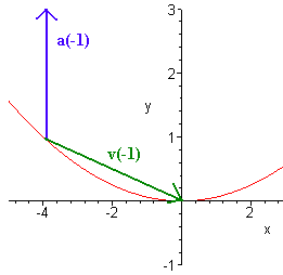
Find the velocity and acceleration of the position function

\[\textbf{r}(t) = (2t-2) \hat{\textbf{i}} + (t^2+t+1) \hat{\textbf{j}} \]

when \(t = -1\). Then sketch the vectors.

Solution

The velocity vector is

\[\textbf{v}(t)= \textbf{r}'(t) = 2 \hat{\textbf{i}} + (2t+1) \hat{\textbf{j}} . \]

Plugging in -1 for \(t\) gives

\[\textbf{b}(-1)= 2 \hat{\textbf{i}} - \hat{\textbf{j}} .\]

Take another derivative to find the acceleration.

\[\textbf{a}(t) = \textbf{v}'(t) = 2 \hat{\textbf{j}} . \]

Below is a picture of the vectors.

Projectile Motion

Since the velocity and acceleration vectors are defined as first and second derivatives of the position vector, we can get back to the position vector by integrating.

Example \(\PageIndex{4}\)

You are a anti-missile operator and have spotted a missile heading towards you at the position

\[\textbf{r}_e = 1000 \hat{\textbf{i}} + 500 \hat{\textbf{j}} \]

with velocity

\[ \textbf{v}_e = -30 \hat{\textbf{i}} + 3 \hat{\textbf{j}} . \]

You can fire your anti-missile at 100 meters per second. At what angle should you fire it so that you intercept the missile. Assume that gravity is the only force acting on the projectiles.

Solution

The acceleration vector of the enemy missile is

\[ \textbf{a}_e (t)= -9.8 \hat{\textbf{j}}. \]

Integrating, we get the velocity vector

\[ \textbf{v}_e (t)= v_1 \hat{\textbf{i}} + (v_2-9.8t) \hat{\textbf{j}} .\]

Setting \(t = 0\) and using the initial velocity of the enemy missile gives

\[ \textbf{v}_e (t)= -30 \hat{\textbf{i}} + (3-9.8t) \hat{\textbf{j}}. \]

Now integrate again to find the position function

\[ \textbf{r}_e (t)= (-30t+r_1) \hat{\textbf{i}} + (-4.9t^2+3t+r_2) \hat{\textbf{j}} .\]

Again setting \(t = 0\) and using the initial conditions gives

\[ \textbf{r}_e (t)= (-30t+1000) \hat{\textbf{i}} + (-4.9t^2+3t+500) \hat{\textbf{j}}. \]

The acceleration of your anti-missile-missile is also

\[\textbf{a}_y(t) = -9.8 t \hat{\textbf{j}} . \]

Integrating, we get the velocity vector

\[\textbf{v}_y(t) = v_1 \hat{\textbf{i}} + (v_2-9.8t) \hat{\textbf{j}}. \]

Since the magnitude of our velocity is 100, we can say

\[\textbf{v}_y(0) = 100 \cos q \hat{\textbf{i}} + 100 \sin q \hat{\textbf{j}} . \]

So that

\[\textbf{v}_y(t) = 100 \cos q \hat{\textbf{i}} + (100 \sin q -9.8t) \hat{\textbf{j}}. \]

Now integrate again to find the position function

\[\textbf{r}_y(t) = (100t \cos q + r_1) \hat{\textbf{i}} + (-4.9t^2 100 \sin q -9.8t + r_2) \hat{\textbf{j}} . \]

Our anti-missile-missile starts out at base, so the initial position is the origin. All the constants are zero.

\[\textbf{r}_y(t) = (100t \cos q ) \hat{\textbf{i}} + (-4.9t^2 100 \sin q -9.8t) \hat{\textbf{j}} \]

Since we want to intercept the enemy missile, we set the position vectors equal to each other.

\[(100t \cos q ) \hat{\textbf{i}} + (-4.9t^2100 \sin q -9.8t) \hat{\textbf{j}} = (-30t +1000 ) \hat{\textbf{i}} + (-4.9t^2 + 3t + 500) \hat{\textbf{j}} \]

Equating coefficients gives

\[ 100t \cos q = -30t + 1000\]

\[ -4.9t^2 + 100t \sin q = -4.9t^2 + 3t + 500 .\]

The first equation gives

\[ t= \dfrac{1000}{100\cos q + 30}. \]

Simplifying the second equation and substituting gives

\[ \dfrac{100000 \sin q }{100\cos q + 30} = \dfrac{3000}{ 100\cos q + 30 } + 500. \]

Clear denominators to get

\[ 100000 \sin q = 3000 + 50000 \cos q + 15000 .\]

At this point we use a calculator to solve for \(q\) to

\[ q = 0.62535 \; rads. \]

Larry Green (Lake Tahoe Community College)

• Integrated by Justin Marshall.